Munich Personal RePEc Archive
Testing Globalization-Disinflation
Hypothesis
Calani, Mauricio
Central Bank of Chile
19 August 2007
Online at
https://mpra.ub.uni-muenchen.de/4787/
Testing the Globalization-Disinflation
Hyphotesis
Mauricio Calani
∗Pontificia Universidad Cat´olica de Chile
Central Bank of Chile
September 8, 2007
Preliminary
Abstract
This paper addresses the globalization - disinflation hypothesis from the perspective of a open economy neo keynesian framework. This hypothesis proposes that globalization has changed the long-run inflation process, resulting in a globaldisinflation. If true, it makes us wonder about the merit of central banks in this phenomenon. Even more, challenges our knowledge that long-run inflation is ultimately a monetary issue. This paper explicitly addresses this hyphotesis, an-alyzing how different degrees of globalization change the response of output and inflation to supply shocks. To accomplish this, the use of a general equilibrium approach in which we can identify and isolate shocks and openness is a must. Globalization is however, a complex process. In this paper I explicitly model globalization just as an open-ness process. Simulation results suggest that as long as there is one distortion - free market for assets, the discussion about the changed values of price stickiness measures which would affect the long-run inflation process is of reduced importance. It is also suggested that financial integration, and not trade or competition, is key to under-standing the link between globalization and inflation.
∗Economist, Economic Research Department, Central Bank of Chile. I thank very
1
Introduction
Why should globalization be an interesting topic to relate with inflation dy-namics? In the last couple of years there has been an outburst of papers which propose a link between globalization and the inflationary process, theoreti-cally as well as empiritheoreti-cally. It would be accurate to say that Kenneth Rogoff began this debate proposing what was later to be called the Globalization-Disinflation Hypothesis, which basically says that globalization has played a strong role in the disinflation process that began in the mid 80’s. Why exactly? The are several features of globalization that would operate in this direction; increased competition makes margins drop marginally, but the ag-gregate effect is large, it also makes it more likely to substitute non tradables for importables which would lead to more flexible prices and after all, when thinking about globalization it is impossible to not think about China and India. Thus, this globalization-led disinflation may have made the task easier for central banks around the world. Data seems to support this idea. In fact, strong central banks as well as very irresponsible and fiscally-dependent cen-tral banks have reached one-digit inflation. At this point of history, chronic inflation has been practically wiped out and now, deflation has caught the attention of researchers.
multiply-ing the positive desired output gap, is actually multiplymultiply-ing zero. This makes less obvious that globalization had something to do with disinflation in coun-tries like the United States or Chile in its openness process in the nineties. And it also makes it less interesting topic to study. However it is interesting to study the implication beyond the non-active inflation bias, in an economy that chooses to pursue an openness process together with firm commitment to price stability.
From the standpoint of the modern monetary theory, inflation dynamics is ultimately a set of decisions taken by price-setting firms. Then, any variable behind long-run inflation should influence the choice firms make or the fre-quency in which they do so. The level of prices firms set, is based on their expectations about marginal costs and desired mark ups, therefore, some-thing must be lowering them systematically for globalization to influence long-run inflation. Put differently, globalization should create expectations of lower future marginal costs for firms to set lower present prices or diminish systematically desired markups through increased competition. The second possibility is that prices are adjusted more frequently than before, because of global competition, a point I will address later.
In this paper I examine carefully these features in a simple model economy that uses the tools of modern monetary theory. I model a economy as sim-ple as possible, keeping only the most basic ingredients that globalization is supposed to change.
I find results that suggest that tariff removal has a relative price adjust-ment process that reduces short-run inflation but that does not change the inflation-process. These results also suggest that while reduced mark ups have an effect on long-run inflation, its magnitude reveals that this reduction cannot be behind global disinflation. The same is true about the frequency of price adjustment.
2
Previous Work
In this section I begin summarizing the debate around the hypothesis that the inflation process has changed due to globalization, and the possibility that this has brought down inflation around the globe. Then I mention recent empirical work that leads to conflicting conclusions, which motivate the idea of dealing with this issue more analytically.
2.1
The debate on the Phillips Curve
Over the past ten years, global inflation has dropped from nearly 30% to low one digit percentages. It has been widely accepted that this trend in infla-tion is due to improved monetary theory implementainfla-tion. Enhanced central bank independence, considerable research on monetary theory and increased public attention to inflation have made central banks around the globe im-prove their practice of monetary policy. Even more, exchange rate crisis have made it clear price stability can only be attained systematically through a solid monetary scheme that commits monetary authority in a credible way. When it comes to inflation, central banks must never stop questioning them-selves about new interesting links between price level determination and other variables. First because it is desirable for them to do so, since that is the only way monetary theory can evolve. And second, because low inflation is a requisite for high sustainable economic growth.
globaliza-tion began a generalized phenomenon. Therefore he is right in his conclusion about the possibility of a steeper Phillips Curve, however it is not clear how this affects inflation in an economy that does not try to attain above-natural output, through systematically expansive monetary policy. This paper seeks to analyze this relation, assuming the model economy does not try to attain a wedge between effective and natural output.
An eloquent answer to Rogoff’s idea was proposed by Ball (2006). He argues that globalization has not reduced the long-run level of inflation, nor has it affected the structure of inflation dynamics. Ball performs analysis to test if the Phillips Curve has actually gotten steeper. He finds that the Phillips Curve in the United States has indeed changed, but in the opposite direction. His estimates are similar to those of Kohn (2006) and he proposes that we should be talking about a flattened Phillips Curve, not a steeper one. In the case of Chile, C´espedes and Soto (2007) find that price rigidity has increased in recent years, and that price indexation to past inflation has decreased. They attribute this finding (flattened Phillips Curve) to increased credibility on Central Bank of Chile’s commitment to price stability. Furthermore, Gal´ı
et al.(2005) estimate New Keynesian Phillips curves relating inflation to real marginal cost and inflation expectations for the United States. They find robust results on their estimations and no evidence of structural change. Thus, who should we believe? Even though Phillips Curves estimations is a common exercise, it is hard to do so; because after all, it entails trying to identify one side of the process that ultimately determines output and inflation. The other component being Aggregate Demand or the Dynamic IS. Even more, the task only gets harder if we consider that this relations vary with productivity shocks. Imagine, for example, aggregate demand is fixed, and the Phillips Curve slope makes it almost vertical; then, if several and large enough productivity shocks move natural output, data would show a group of observations around a determined level of inflation, and estimates of Phillips Curves would suggest a flattened relationship.
Given the uncertainty of the real Data Generating Process, it is hard to tell which estimates are correct1. This is the basic reason of choosing a more
analytical framework to analyze the extend to which globalization can affect inflation and output dynamics.
In section 4 I examine analytically diverse channels through which global-ization could affect the output-inflation trade-off sufficiently to explain the global disinflation phenomenon. I discuss the role of mark ups, competition,
1
price flexibility and tariff removal as possible sources for this phenomenon. Thus it is important to make a few comments on the output-inflation trade-off (if it exists at all) which I do next.
2.2
Choosing (non) neutrality of money
The Keynesian economics development during the 80’s was an attempt to provide micro foundations to key Keynesian features and assumptions. Mod-els in this literature suggest non-neutrality of money. Menu Costs, Staggered Contracts, and other models were widely studied to explain money short run non-neutrality. However these models were static and made no connection with other features of the economy. On the other hand, the Real Business Cycle literature emphasized the irrelevance of monetary policy and proposed technology as the main source of economic fluctuation. Money could be in-cluded but it remained neutral. The New Keynesian counter revolution was a natural result of this lines of research. NK models emphasize the role of price setting and money non-neutrality adopting the RBC methodology. As mentioned before, the debate on the effects of globalization on inflation process has focused attention in key structural parameters of the New Key-nesian Framework, this it is natural to use it to examine such propositions. Real Business Cycle work has been previously done for Chile, worthy exam-ples are Duncan (2005) and Ochoa and Valenzuela (2005). Models in this literature included money, but it remained neutral. This is a natural result of including a Sidrausky-type utility function and no nominal rigidities. Indeter-minacy of price level is also a characteristic of this type of models. Woodford (2003) makes an excellent analogy for the price level indeterminacy. He says that in the classical growth model, real variables can be thought of as a pen-dulum, which after shocks returns to the initial steady state level; however, nominal variables can be thought of as a cylinder that once moved, can reach an indeterminate new steady state.
3
The Model
The dynamic stochastic general equilibrium model to be used has to explic-itly consider several features in the transmission mechanism of the monetary policy. I model the Chilean economy as stationary. It is not difficult to show that results are not different from those obtained from a model with trend exogenous growth, since we can always de-trend the equilibrium paths of en-dogenous variables. Furthermore, Chilean growth dynamics are more likely to to be consistent with deterministic trends, and thus exogenous growth models, as shown by Chumacero and Fuentes (2006). Besides, there is no reason to think that trend growth has a relation with inflation, since if there is any relation at all between these, we should suspect inflation to be related to the business cycle and not to the trend. The framework I use departs from the Real Business Cycle literature assuming nominal and real rigidities that make monetary policy non neutral. This model also incorporates distortions, which make the steady state inefficient. However, I suppose the monetary authority does not try to solve this inefficiency through systematically ex-pansive monetary policy since it is not realistic and it is not the focus of this paper.
3.1
Households
This economy is inhabited by a representative, infinitely lived household that maximizes
Et
∞
X i=0
βtU(cm,t, ch,t,
Mt
Pht
) (1)
where Et denotes the mathematical expectations operator conditional on
information available at time t, β ∈ (0,1) represents a subjective discount factor, andU is a period utility index assumed to be strictly increasing in its arguments, and strictly concave. Specifically,cm,trepresents the consumption
of importable goods, ch,t is the level of consumption of the composite non
tradable goods and Mt is the quantity of money held by the household in
period t. Of course, Ph,t is the price level of the non tradable composite
good. The consumption good is assumed to be a composite made up of a continuum of differentiated goods ch,t(i) indexed by i ∈ [0,1] via the CES
aggregator
ch,t = [ Z 1
0 ch,t(i) 1−1
η
di]
1
1−1η (2)
optimally, it will seek to maximize the level of ch,t given a total expenditure R1
0 ph,t(i)ch,t(i)di, therefore it solves
maxch,t = [ Z 1
0 ch,t(i) 1−1
η
di]
1 1−1η
+µ[zt− Z 1
0 ph,t(i)ch,t(i)di]
(3)
where the first order condition associated is
c
1 η
h,tch,t(i)
−1
η =µp
h,t(i) (4)
that must hold for allch,t(i) and also for the basket as a whole: ch,t, obtaining
ch,t(i) =
ph,t(i)
ph,t !1−η
ch,t (5)
Remember that total expenditure is given by zt = R01ph,t(i)ch,t(i)di and if
there is an index so that zt =ph,tch,t then
ch,t(i) =
ph,t(i)
ph,t !−η
zt
ph,t !
Z 1
0 ph,t(i)ch,t(i)di =
Z 1
0
ph,t(i)
ph,t !1−η
ztdi
ph,t = Z 1
0 ph,t(i) 1−η
di
1−1η
(6)
Thus, once the demand for the composite good cht is determined, it is
easy to obtain demand for variety i.
The budget to which the consumer is constrained is given by
pm,t(1 +τm,t)cm,t+ph,tch,t + (1 +τm,t)pm,tit+
bt+1
1 +rt
+ (1 +Rt)(1 +et)Dt∗+Mt−1 ≤vtpm,t(1 +τm,t)Kt+Mt
+bt+Dt∗+1+ Υt+ Φh+ Φx (7)
where τm,t represents the import tariff, cm,t is the consumption of
importa-bles, it investment, bt stands for total government bonds (nominal) held by
households, rt is the nominal interest rate, Rt is the external interest rate,
et is the appreciation (depreciation) of the nominal exchange rate, D∗t
lump sum taxations (subsidies), finally, Φh and Φx represent profits from the
non-tradable good technology and exportable good technology respectively. The capital law of motion is given by
Kt+1 = (1−δ)Kt+it (8)
The problem of the representative consumer can be summarized by the value function that satisfies:
V(sh) = max (U(ch,t, cm.t,
Mt
Ph, t
) +βE[V(sh+1)]) (9)
subject to (7) and (8) and the perceived law of motion of the state variables. if the functional form of the instant utility function is given by
U(cm,t, ch,t,
Mt
Ph,t
) = 1
1−σ
c
ϕ m,tcγh,t
Mt
Ph,t
!1−ϕ−γ
1−σ
(10)
where σ is the constant relative risk aversion coefficient 2. Then the first
order conditions for the consumer are given by
1 = ϕ
γ
cm,tpm,t(1 +τm,t)
ch,tph,t
Mt =
1−ϕ−γ
ϕ cm,tpm,t(1 +τm,t)
r t
1 +rt −1
β(1 +rt) =
ch,t+1ph,t+1 ch,tph,t
(1 +rt) = (1 +Rt)(1 +et)
1 +vt+1−δ =
1
β cm,t+1
cm,t
(11)
The first equation is the intra temporal condition, the second relates money to consumption and interest rate. There are two observations worth mentioning about this condition, first, it comes from a Sidrausky-type util-ity function in which money is held as a store of wealth, which is simpler than modeling cash-in-advance constraints; second, money demand depends inversely of rt
1+rt, which is consistent to the observation Easterlyet. al make,
arguing this is the true cost of money in contrast to typical money demand equations that relateMttolog(rt) or simply tort. The third condition is the
Euler equation, the fourth is the uncovered interest parity condition. Finally, the last condition relates the marginal gain of investing in capital and the inter temporal rate of substitution.
2
3.2
Firms
As one can notice, the consumer’s budget constraint includes two types of goods that are not the same as those in the instant utility function (10) because the consumer does not consume exportable goods, but sells them abroad and perceives a rent for them. The production of these goods will be determined by foreign demand, more specifically, by the observed inter-national price. Both, exportable and non tradable goods are produced with a technology that requires only capital, which as Chumacero et al. (2004) notice is consistent with a model in which labor is sector specific. This as-sumptions greatly reduces computational work and is not determinant to the results, since there is no obvious way globalization affects or is affected by la-bor dynamics. In practice, lala-bor market is important to inflation forecasting because labor costs tend to be a leading indicator of inflationary pressure, however in this model I explicitly model marginal cost, thus there is no loss of generality and simplicity is kept. Importables are not produced in the coun-try, I assume the sector that substitutes importables for national production is nil.
3.2.1 Non Tradables
Each good’s varietyi∈[0,1] is produced by a single firm in a monopolistically competitive market. Each firmiproduces output using only capital,ki,t with
a production function given by
ezh,tF(k
i,t)
where I assume F to be concave, and strictly increasing in capital. The variable zh,t denotes an stochastic productivity shock common to all firms
in this sector. The firm takes into account the monopolistic competition environment when deciding price setting. Each variety is produced by a firm, therefore every firm faces a demand (absorption) equal to ah,t(i) =
ch,t(i) +χgt(i), where again, gh,t(i) = p
h,t(i)
ph,t
−η
χgt
ah,t(i) =
ph,t(i)
ph,t !−η
ah,t
thus, every firm must maximize
φh,t(i) =ph,t(i)
ph,t(i)
ph,t !−η
but it also knows that prices are sticky `a la Calvo. More specifically only a fraction 1−θof firms are allowed to adjust prices optimally every period. Thus the actual objective function to maximize is the discounted profit subject to the constraint that every firm must satisfy demand in every period.
maxEs
∞
X s=t
1 1 +rt,s
!s−t
θs−t
(
p∗h,tYs|t−vs(1 +τm,s)pm,skh,s+
¯
mc ezh,skαh
h,s(i)−(
p∗h,t ph,s
)−ηah,s(i) ! )
(12)
The first order condition associated to ph,t and kh,t
∞
X s=t
1 1 +rt,s
!
θs−tYs|t
p∗h,t ph,s
− η
η−1mcs
!
= 0
vt(1 +τm,t)pm,t−ph,tmctαhezhtkαh,th−1 = 0 (13)
It is clear from these equations that the price setting decisions taken by firms depend on the expectation of mark ups, which depend on the expectation of future prices and marginal costs. The first condition in (13) can be ex-pressed in two parts,x1t andx2t, wherex1t =P∞
s=t
1 1+rt,s
θs−tph,t(i)∗
ph,s
1−η
ah,s
and x2t = P∞ s=t
1 1+rt,s
θs−tph,t(i)∗
ph,s
−η
ah,sMM Cs, holding x1t = x2t at all
times. Notice that this auxiliary variables can be recursively expressed as
x1t =
p∗
h,t
ph,t
1−η
at +
p∗
t
p∗
t+1
1−η
θ
1+r
x1t+1 and xtr = atMM Ct p∗ h,t ph,t −η + θ 1+r p∗ h,t p∗ h,t+1 −η
x2t+1.Since the probability that each firm re-sets prices is 1−θ, then
ph,t1−η =θph,t1−−η1+ (1−θ)p1h,t−η (14)
3.2.2 Tradable Goods
The technology in this sector
f(zx,t, kx,t) = ezx,tkx,tαx (15)
So the problem to solve by this firm (which doesn’t face monopolistic com-petition) is;
maxφx = (1−τx,t)qezx,tkx,tαx −vtpm,t(1 +τm,t)kx (16)
The first order associated condition is
Notice that there are neither nominal nor real rigidities in this sector. In the Chilean case there is vast literature analyzing whether or not copper industry has any monopolistic position in world market and most studies tend to use terms like modest or limited, therefore I choose to model this sector of the economy as perfectly competitive, facing terms of trade. I assume that the productivity shocks(zi) follow AR(1) processes:
zj,t+1 = (1−ρj)¯zj,t+1+ρjzj,t+υj,t+1
υj,t+1 ∼ N(0, σj2) (18)
3.3
Government
Government is composed by two separate institutions, fiscal government and a monetary authority.
3.3.1 Fiscal Authority
I model fiscal authority in a very simple and popular way. Government does not try to influence the economy through subsidies or taxes meant to solve for the monopolistic competition inefficiency. It limits itself to fulfill
τm,t(cm,t+it) +
bt+1
1 +r −bt≥gt+ Υt (19)
I assume there is a fiscal component that is predetermined. I follow Chu-macero et al. (2004) assuming the following autoregressive process:
lngt+1 = (1−ρg)¯gt+1+ρglngt+υg,t+1
υg,t+1 ∼ N(0, σg2) (20)
3.3.2 Monetary Authority
Monetary Policy is modeled in a widely accepted way, to concentrate on the issues of the openness and not the rule chosen.
ln(1 +rt+1) =ρM Pln(1 +rt) + (1−ρM P)(ln(1 + ¯r) +
ρπln(
pht+1
ph ) +ρyln( Yt
Yn)) (21)
3.4
External Sector
I follow Schmitt-Groh´e and Uribe (2003) to determine the external rateRt=
¯
faced by domestic agents, Rt, is increasing in the aggregate level of foreign
debt, ˜d. Specifically I assume the functional form assumed by Chumaceroet al. (2004)
Rt+1 = (1−ρr) ¯Rt+1+ (1−ρr)Ω(
D∗t yt
) +ρrRt+υR,t+1
υR,t+1 ∼ N(0, σR2) (22)
I also assume that terms of trade are exogenously given.
lnqt+1 = (1−ρq)qt+1+ρqlnqt+υq,t+1
υq,t+1 ∼ N(0, σ2q) (23)
3.5
Market Clearing
The capital market must empty. In this highly stylized economy all capital is imported and is demanded only by the two sectors that produce final goods: The non tradable sector and the exportable sector.
Kt=kx,t+kh,t (24)
Notice the relation between current account and capital account: −Dt∗+1+
D∗t = (1− τx)qyx −cm,t −(1 −χ)gt − kt+1 + (1 −δ)kt −RtDt∗ There is
no need to empty the exportable sector since the price (terms of trade) has been exogenously given. However it is necessary to empty the non tradable market. Remember that the composite good ch,t is aggregated according to
ch,t = [R01cih,t
1−1 ηdi]
1
1−1η and that the market for every variety i∈ [0,1] must
empty: f(zh,t, kh,t(i)) = ah,t p
h,t(i)∗
ph,t
−η
where, as was previously defined:
ah,t = (ch,t(i) +χgh,t(i)) If we defineyh,t =R01f(·)(i) then,
f(zh,t, kh,t) = ah,t Z 1
0
ph,t(i)∗
ph,t !−η
di
st = Z 1
0
ph,t(i)∗
ph,t !−η
di (25)
st of the form:
st = (1−θ)
ph,t(i)∗
ph,t !−η
+ (1−θ)θ ph,t−1(i)
∗
ph,t
!−η
+θ2(1−θ) ph,t−2(i)
∗
ph,t
!−η
+· · ·
(26)
And once again it is possible to obtain a recursive expression to model the variable st. As Schmitt-Groh´e and Uribe (2007) notice, this variable is a
measure of price dispersion that is in the unity neighborhood. Sadly, most work done in this framework assume that this dispersion term can be ac-curately approximated to unity. However, since it modifies the aggregation condition, small deviations create big distortions that can seriously change results. Thus I choose not to approximate it.
st+1 = (1−θ)
ph,t(i)∗
ph,t !−η
+θ ph,t ph,t+1
!−η
st (27)
3.6
Calibration
Since the objective of this paper is analytical, I consider important to fol-low well accepted parameter values for the Chilean economy. This way, it is less likely that criticism around parameter values causing results take place. There are several contributions to real business cycle literature for the Chilean economy. Perhaps the most important ones are Chumacero et al. (2004), Chumacero and Fuentes (2006), Caputo et al (2007), Bergoeing and Soto (2002) and Duncan (2005). Microeconomic studies are scarce, and is is worth emphasizing recent work by Medina et al (2006) on micro - price dynamics.
Symbol Value
β 0.992
η 5.7
ϕ 0.6813
γ 0.2187
δ 0.025
αx 0.45
αh 0.3
¯
zx 4.90
¯
zh 2.76
¯
Symbol Value ¯
g 1.773
¯
q 0.25
τm 0.02
τx 0.051
χ 0.92
Parameters were taken from previous studies and modified when necessary to make them consistent to quarterly model. AR(1) processes described in this section are assumed to have the following parameters: ρR = 0.9; ρg = 0.8;
ρq = 0.86; ρx = 0.9, ρh = 0.9. Most of this AR(1) parameters were taken
from Chumacero et al (2004) which is one of the few studies that calibrate parameters to analyze openness in Chile. Finally, σx = 0.001, σh = 0.01,
σq = 0.01, σR = 0.001. Next section presents the results of some simulations
and insights that can be drawn from them
4
Results
As I argued previously, I do not use log linearizations to solve the model numerically. I however, use a perturbation method proposed by Schmitt-Groh´e and Uribe (2004), which has been proven to outperform usual linear quadratic method solutions. The equations that determine the equilibrium in the model can be expressed in two groups, xt is a vector of predetermined
variables (endogenous and exogenous) and yt represents not predetermined
variables. The same is true about xt+1 and yt+1. All first order conditions
can be expressed in a system that takes the form:
Etf(yt+1, yt, xt+1, xt) = 0,
where Et denotes the mathematical expectations operator conditional on
information available at time t. Policy functions, as usual, depend only on state variables: yt=g(xt), xt+1 =f(xt). Next, I present the results of some
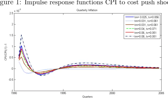
Figure 1: Impulse response functions CPI to cost push shock
Source: Author’s calculation
Quarterly inflation of consumer prices (includes nontradables and importables weighted by their spending share in total consumption)
4.1
Supply shocks and tariff removal
If different degrees of openness can affect the inflation dynamics process, then the same supply shock, everything else equal (included the monetary regime), should have a different impact on the economy. Furthermore, inflation dy-namics should be particularly sensitive to openness to be able to explain inflation downwards trend. Figure (1) shows different responses of inflation dynamics to the equivalent of a one percent shock to marginal cost. This shock hits the productivity of non-tradable technology with a one standard-deviation negative shock. As can be seen from figure 1, it is true that differ-ent combinations of tariffs can have an effect in inflation dynamics, but since these affects mostly relative prices and resource assignation, openness has more relation to the very steady state and not so much with the dynamics when the economy is hit by cost push shocks3. Thus, the inflationary process
is affected by the degree of openness. The more open the economy (in term of tariffs) the smaller the impact is on the consumer price index. The relation is not linear though, since the mechanism is complex. It is important to notice the differences though. Very closed economies (8% of import tariff) do not exhibit larger enough responses than very open economies (2,5% of import tariff). This is not surprising, since tariffs affect relative prices, not the general level of prices, that is captured by CPI. Even more, as I mentioned in
3
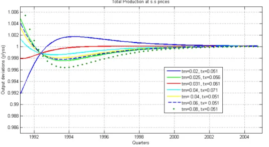
Figure 2: Impulse response functions of output deviation to cost push shock
Source: Author’s calculation
Deviation from natural level of output for different degrees of openness
the introduction. For a variable to influence the inflation dynamics process it should have some influence on the prices firms set or the frequency they do so. Tariffs have no relation with the schedule of price setting, and have a lim-ited effect on the prices firms set. Therefore tariff removal and trade growth, while having a huge impact on welfare and efficiency4, have no effect on
long-run inflation. Figure 2 shows the impulse response functions for output5. An
interesting caveat is in place. China and India have gained protagonism in world trade. This has led many authors to say that they are exporting de-flation and globalization has made it easier for other countries to benefit from it. I believe this is theoretically wrong. China and India are countries characterized for having low labor cost which enables them to export low cost final goods. In the “accountability” perspective of inflation this leads to cheaper consumer baskets and to lower inflation. However this is a relative price matter. Imagine a world in which there are no countries but individual producers. One of them discovers a way to make one good cheaper. Of course CPI in the near future will be lower, because relative prices have changed, but they do so until they find their new equilibrium in which marginal rates of substitution equal new relative prices. Relative prices, however, cannot change systematically downwards or upwards. Thus the China phenomenon
4
Excellent studies about the gains from increased trade in Chile are Chumacero et al.
(2004), Coeymans and Larra´ın(1994) and Harrison (2005)
5
has indeed some effect on global “accounting inflation” but has not changed at all the inflationary process, which is ultimate source of long-run inflation. Summarizing, trade removal has effects on relative prices and not the infla-tionary process. Furthermore, this effect is small enough not to be relevant in the disinflation trend many countries have experienced. Next sub-section examines another feature of globalization: Increased Variety and its relation to marginal costs.
4.2
Variety, Marginal Costs and Inflation dynamics
In this section a similar experiment is done. However, the changing parameter is η. Remember that in steady state the optimal markup for nontradable firms is given by M. This comes from the first order condition associated to decision of price setting.
∞
X s=t
1 1 +rt,s
!
θs−tYs|t
p∗h,t ph,s
− MM Cs !
= 0
In steady state p∗h,t
ph,s equals 1. ThereforeM CsM = 1 should hold. In steady
state, no firm wants to change prices, thus M is the desired mark up. As
mentioned before, M= η
η−1 depends on the elasticity of substitution in the
CES aggregator. Whenη(>1) approaches∞non tradable varieties are more likely to substitute one another when prices change. In microeconomic prin-ciples, the larger η is, the larger the ratio ∂ln(ci/cj)
∂ln(pj/pi), meaning the easier it is
to substitute one variety for another.
Why should η change? Recall the Hotelling analogy, in which monopolis-tic competition takes place by differentiated products that are distant one another. If variety has increased, the distance between one variety and an-other is reduced, and the possibility to substitute one good for anan-other is increased. How can we introduce this feature in the model? By changing the parameter η upwards. This has another implication. Ifη is higher, then M, the desired mark up falls. ∂∂ηM = (η−11)2. This result is consistent intuitively
and theoretically.
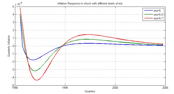
As seen by figure (3) the lowerη is, the higher the desired markup is too. This creation of variety is indeed making the NKPC steeper. And proper values of η change inflation dynamics. Thus, after all, globalization does change inflation dynamics. However it is important to notice that ∂∂η2M2 =
− 2
(η−1)3 and that elasticity η can not change but marginally. Thus, even if
Figure 3: Impulse response functions of output deviation to cost push shock
Source: Author’s calculation
Quarterly inflation in response to supply shock and different levels of elasticity of substitution across non tradable varieties.
the effect on inflation would dissapear. What is left then? The most obvious parameter in the neo keynesian framework: θ. Next I analyze its effects.
4.3
Price stickiness and Capital Account
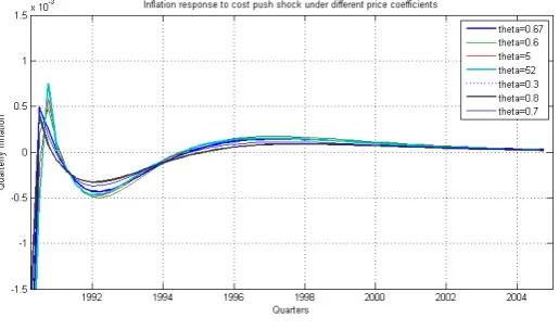
The same experiment is done to different values of θ. This is the Calvo co-efficient that is a measure of price stickiness. Every period a firm set a new price with probability equal to 1−θ. On average, a firm re-sets its price every
1
1−θ periods. A very accepted value for the Chilean economy is 0.667, which
Figure 4: Impulse response functions of inflation to cost push shock with different degrees of price stickiness
Source: Author’s calculation
Quarterly inflation in response to supply shock and different levels ofθ.
the stochastic component of productivity in the non-tradable sector. This magnitude explains the big variations on debt to output ratio. This effect is magnified by the incapability of prices to adjust quickly to optimal levels.
Figure 5: Debt / GDP ratio variation
Source: Author’s calculation
Quarterly inflation in response to supply shock and different levels ofθ.
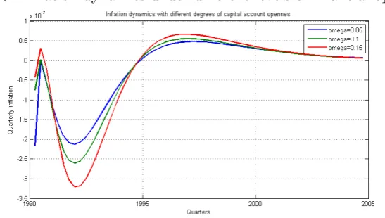
Figure 6: Inflation dynamics under different levels of financial openness
Source: Author’s calculation
[image:22.595.161.435.481.636.2]Figure 7: Foreign debt under different levels of financial openness
Source: Author’s calculation
Deviation from steady state in response to supply shock and different values ofω.
Notice that the largest effects obtained so far, were those of variations of price stickiness coefficient. However very lowvariations on the coefficient Ω, measuring financial openness, can accomplish variations in inflation 10 times larger. Thus it is not surprising that the Mundell Fleming model emphasized the importance of capital account openness without the use of a DSGE.
5
Concluding Remarks
References
[1] Ball, L. 2006. “Has Globalization Changed Inflation”. NBER Working Paper 12687.
[2] Barro, R. and D. Gordon. 1983. “A Positive Theory of Monetary Policy in a Natural Rate Model”. Journal of Political Economy 91(4):589-610. [3] Batini, N., D. Laxton. 2007. “Under What Conditions can Inflation Targeting be Adopted? The Experience of Emerging Markets. In Mon-etary Policy under Inflation Targeting”, edited by F. Mishkin and K. Schmidt-Hebbel, 1-22. Santiago: Central Bank of Chile.
[4] Batini, N., R. Harrison, S. Millard. 2003. “Monetary policy rules for an open economy”. Journal of Economic Dynamics & Control 27: 2059-2094.
[5] Belaygorod, A. and M. Dueker. 2005. “Discrete Monetary Policy Changes and Changing Inflation Targets in Estimates Dynamic Stochas-tic General Equilibrium Models”.Federal Reserve Bank of St. Louis Re-view”,87(6), 719-33.
[6] Bergoeing, R. y R. Soto. 2002. “Testing Real Business Cycle Models in an Emerging Economy.” Working paper 159. Central Bank of Chile.
[7] Calvo,Guillerno. 1983. “Staggered Prices in a Utility Maximizing Frame-work” Journal of Monetary Economics 12:383-398.
[8] Caputo, R. F. Liendo and J. P. Medina. 2007. “New Keynesian Models for Chile in the Inflation-Targeting Period. In Monetary Policy under Inflation Targeting”, edited by F. Mishkin and K. Schmidt-Hebbel, 1-22. Santiago: Central Bank of Chile.
[9] C´espedes, L. and C. Soto. 2007. “Credibility and Inflation Targeting in Chile”. In Monetary Policy under Inflation Targeting”, edited by F. Mishkin and K. Schmidt-Hebbel, 1-22. Santiago: Central Bank of Chile.
[10] Chumacero, R. and R. Fuentes. 2006. “Chilean growth dynamics”. Eco-nomic Modelling, 23: 197-214.
[12] Chumacero, R., J.R. Fuentes, K. Schmidt-Hebbel. 2004. “Chile’s Free Trade Agreements: How Big is the Deal?.” Working Paper 264. Central Bank of Chile.
[13] Coeymans, J.E. y F. Larran. 1994. “Efectos de un Acuerdo de Libre Comercio entre Chile y Estados Unidos: Un Enfoque de Equilibrio Gen-eral”Cuadernos de Econom´ıa, Vol. 31, No. 94, pp. 357-400.
[14] Duncan, R. 2005. “How Well Does a Monetary Dynamic Equilibrium Model Account for Chilean Data?”.General Equilibrium Models for the Chilean Economy”, edited by R. Chumacero and K. Schmidt-Hebbel, 261-301.Santiago: Central Bank of Chile.
[15] Gali, J., M. Gertler, J. L´opez-Salido. 2005. Robustness of the estimates of the hybrid New Keynesian Phillips curve. Journal of Monetary Eco-nomics 52: 1107-1118.
[16] Ihrig, J. S. Kamin, D. Lindner, J. Marquez. 2007. “Some simple Tests of the Globalization and Inflation Hypothesis”. Internacional finance Discussion Papers, 891. Federal Reserve System.
[17] Mankiw, G. 2001. “The Inexorable and Mysterious Tradeoff Between Inflation and Unemployment”. The Economic Journal, 111, May. [18] Mishkin, F. and K. Schmidt-Hebbel. 2007. “Monetary Policy under
In-flation Targeting: An Introduction”. InMonetary Policy under Inflation Targeting”, edited by F. Mishkin and K. Schmidt-Hebbel, 1-22. Santi-ago: Central Bank of Chile.
[19] Mishkin, F. and K. Schmidt-Hebbel. 2007. “Does Inflation Targeting Make a Difference”. In Monetary Policy under Inflation Targeting”, edited by F. Mishkin and K. Schmidt-Hebbel, 1-22. Santiago: Central Bank of Chile.
[20] Ochoa, M. and P. Valenzuela. 2004. “Impactos de un Shock Externo en un Modelo Estoc´astico de Equilibrio General para una Econom´ıa Abierda: El caso de Chile”. manuscript, Universidad de Chile.
[21] Schmitt-Groh´e, S. and M. Uribe. 2003. “Closing Small Open
Economies”. Journal of International Economics 61:163:185.
[23] Schmitt-Groh´e, S. and M. Uribe. 2004. “Solving dynamic general equilib-rium models using a second-order approximation to the policy function”.
Journal of Economic Dynamics & Control” 28:755-775.
[24] Schmitt-Groh´e, S. and M. Uribe. 2007. “Optimal Inflation Stabilization in a Medium-Scale Macroeconomic Model”, In Monetary Policy under Inflation Targeting”, edited by F. Mishkin and K. Schmidt-Hebbel, 1-22. Santiago: Central Bank of Chile.
[25] Rogoff, K. 2003a. “Globalization and Global Disinflation”. Paper pre-pared for the Federal Reserve Bank of Kansas City, Jackson Hole.
[26] Rogoff, K. 2003b. “Disinflation: An Unsung Benefit of Globalization?”.
Finance and Development 2003. IMF.
[27] Taylor, J. 2006. “Implications of Globalization for Monetary Policy”.