Munich Personal RePEc Archive
Macroeconomic framework for the
economy of Bangladesh
Khondker, Bazlul Haque and Raihan, Selim
South Asian Network on Economic Modeling (SANEM),
Department of Economics, University of Dhaka, Bangladesh
May 2008
M
M
A
A
C
C
R
R
O
O
E
E
C
C
O
O
N
N
O
O
M
M
I
I
C
C
F
F
R
R
A
A
M
M
E
E
W
W
O
O
R
R
K
K
F
F
O
O
R
R
T
T
H
H
E
E
E
E
C
C
O
O
N
N
O
O
M
M
Y
Y
O
O
F
F
B
B
A
A
N
N
G
G
L
L
A
A
D
D
E
E
S
S
H
H
Bazlul Haque Khondker and Selim Raihan
May 2008
CONTENTS
LIST OF ABBREVIATIONS iii
KNOWLEDGE SUMMARY 1
CHAPTER 1 3
BACKGROUND 3
CHAPTER 2 4
A BRIEF ASSESSMENT OF EXISTING ‘FINANCIAL’ PROGRAMME AT MOF 4
CHAPTER 3 6
PROPOSED MODIFICATION TO EXISTING FRAMEWORK 6
CHAPTER 4 7
SPECIFICATION 7
CHAPTER 5 30
DATA AND PARAMETERS 30
CHAPTER 6 31
MODEL ESTIMATES VERSUS DATA 31
CHAPTER 7 32
MACRO OUTLOOK: TREND SCENARIO 32
POVERTY OUTLOOK: TREND SCENARIO 33
CHAPTER 8 35
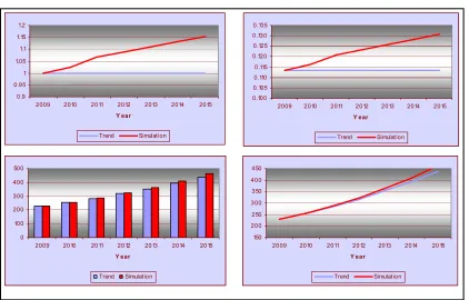
SCOPE OF SIMULATION 35
CHAPTER 9 36
SIMULATION DESIGN 36
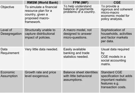
ANNEX = 1: MODEL COMPARISON 38
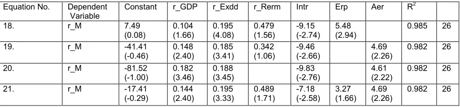
ANNEX = 2: RESULTS OF REGRESSION 39
ANNEX = 3: SOME TAX REVENUE SOURCES AND THEIR PROXY BASES 41
ANNEX = 4: ACKNOWLEDGEMENT 42
ANNEX = 5: TERMS OF REFERENCE (TOR) 43
LIST OF TABLES:
Table 1: Simulation Design and Impact ... 37
Table 2: Framework Comparisons ... 38
Table 3: Regression Results Private Consumption ... 39
Table 4: Regression Results Private Investment ... 39
Table 5: Regression Results Export ... 40
Table 6: Regression Results CPI ... 40
Table 7: Regression Results Import ... 40
LIST OF FIGURES: Figure 1: Linkage between Fiscal side and Money side... 23
LIST OF ABBREVIATIONS
ADB Asian Development Bank
ADP Annual Development Programme
BBS Bangladesh Bureau of Statistics
CGE Computable General Equilibrium
CPI Consumer Price Index
FMRP Financial Programming Reform Project
FPM Financial Programming Model
ICOR Incremental Capital Output Ratio
MOF Ministry of Finance
MTMF Medium Term Macro Economic Framework
NBR National Board of Revenue
PSBR Public Sector Borrowing Requirement
RMSM Revised Minimum Standard Model
SAM Social Accounting Matrix
KNOWLEDGE SUMMARY
The Asian Development Bank (ADB) provided support to the MOF to formulate a user: friendly and easily transferable computable general equilibrium (CGE) model to reflect the effect of changes in various public policies and forecast changes of fiscal policy on different sectors of the economy. However, given the difficulties posed by institutionalization of the CGE model and the priorities of the Finance Division, it was agreed that the modeling exercise should be compatible with the financial programming framework. Furthermore, it was agreed that the consultant team would improve the existing macro:economic framework maintained by the Finance Division. In accordance to their recommendation, the following features are added to the existing framework.
• Introduce behavioral specifications for some key variables — namely production behavior, revenue functions, capital formation, private investment functions, private consumption etc.
• Improve the interdependence between variables of different blocks namely between real side and government budget; government budget, money and BOP; money and real side.
• Introduce policy instruments to expand the simulation possibility. The range of instruments may include direct and indirect tax rates, tax base, subsidy, exchange rates etc.
• It is argued that the transfer of technology to run the proposed model partly depends on the simplicity and user’s friendly feature. Although, the simplification limits the simulation capability of the model, considering the important objective of technology internalization the model will be constructed in an ‘Excel’ spread sheet.
• The following provides specifications of the macro:economic framework. In accordance to the existing practice, the macro:economic framework contains blocks: Real side; Government Budget; Money; and Balance of Payment. In addition to these blocks, a debt block is appended to capture debt dynamics.
Data period considered in this framework is 2002 to 2007. Almost all data used in the macro:economic framework has been provided by the Finance Division and the FMRP project. Breakdown of value added (i.e. GDP) by labor value added and capital value added was obtained from the updated social accounting for Bangladesh for 2005. World Economic Outlook forecasts were reviewed to get parameters for external sector (e.g. world price of imports and exports, world inflation rate etc.).
It is important to note from the objective and purpose of the ‘financing programming’ that, it is essentially a framework to assess the financing options in accordance to a targeted economic growth and inflation rate. In contrast to the simulation feature of a CGE model, it is primarily an accounting framework limiting the scope to conduct policy simulations. Moreover, it is specified at the macro level restricting the scope of sectoral impacts analysis and output generation. Despite its’ limitation as a simulation framework, a number of scenario generation capabilities are incorporated. A possible list of policy simulations available in the framework is given below:
• Altering indirect tax bases (both domestic and external) various types of indirect tax bases. For instance, these may include bases of VAT, excise duty, import duties, supplementary duty, and all other taxes.
• Expanding direct tax bases by raising the threshold, reducing the exemption and deduction levels.
• Changing the direct tax rates. For instance, these may include personal income tax rates, and corporate tax rates.
• Expanding non:tax revenue sources.
• Expanding the coverage of the government expenditure program both re:current and capital. For instance, full or partial indexing of pay:allowance item to CPI.
• Re:setting world price of imports.
• Re:setting the growth rates of various components of money and credit. They include private credit growth; net other asset growth etc. Variations in them affect net domestic assets leading to changes in money supply.
• Re:setting the growth rates of various balance of payment. For example, they include current transfer; loan disbursement, grant disbursement. Variations in them affect current account balance and resources for deficit:financing implicating the requirement for bank borrowing.
CHAPTER 1 BACKGROUND
The Asian Development Bank (ADB) provided support to the MOF to formulate a user friendly and easily transferable computable general equilibrium (CGE) model (more specifically a macro:economic framework) to reflect the effect of changes of various public policies and forecast changes of fiscal policy on different sectors of the economy. In this context two rounds of meetings took place between the consultant team and the officials of the MOF before the implementation of the framework. The first meeting was held on 22 January 2008 where Mr. Arastoo Khan, Joint Secretary, MOF introduced the consultant team to the officers of the budget wing and reviewed the different elements of the Terms of Reference (TORs). During the meeting it was discussed that a CGE model is different from the financial programming frameworks of the Bank1 and the Fund2 with respect to objective, structure, data need, simulation possibility and outcomes. Moreover, the features of these two different types of frameworks (i.e. CGE and financial programming) usually are not possible to accommodate into an integrated framework. This aspect was pointed out by the consultant team during their meeting with the Finance Division. Considering the above: mentioned difficulties and the priorities of the Finance Division, it was agreed that the modeling exercise will be compatible with the financial programming framework. Thus it was agreed that the first item of the TORs will not be covered in the study. Other item of the TORs will be retained. It was further decided to add features to the exiting macro:economic framework of the MOF. Accordingly a review of the macro:economic framework of the MOF involving the consultant team and the officials of budget wing was proposed. An in:depth review of various components of the MOF framework took place on 29 January 2008. Md. Abdur Rahim Khan and Md. Habibur Rahman, Senior Assistant Secretary, MOF presented the MOF macro:economic framework to the consultant team.
1 The Bank’s model examines the overall amount of resource that a country required to meet its target economic growth rate. Having estimated likely investment from domestic taxation and savings plus foreign investment it determines how much additional finance is required from development agencies. The so called “financing gap” is then filled by aid grants and loans.
CHAPTER 2
A BRIEF ASSESSMENT OF EXISTING ‘FINANCIAL’ PROGRAMME AT MOF
The MOF in Bangladesh, among others, is entrusted to formulate short and medium development plans to enhance welfare and reduce poverty of the people. The short:term plan and the medium term plans are respectively known as the annual budget and medium term macro economic framework (MTMF). The Budget wing of the MOF has been maintaining a Macro:economic Framework to assist the preparation of short and medium term macro:economic frameworks. The framework falls into the well:known class of financial programming framework used by the Bretton Woods institutions. The framework consists mainly of four major blocks: (i) Real Side; (ii) Government Budget; (iii) Money and Credit; and (iv) Balance of Payment. In addition to these four blocks, the MOF framework contains few extra worksheets to assist a more thorough understanding of the expenditure budget and preparation of the monetary survey component. Moreover it shows projection of sectoral GDP. The sector classification follows the sector classification adopted the Bangladesh Bureau of Statistics (BBS).
An examination of resource requirement consistent with the target growth rate is the starting point. Once the policy:makers/analysts reach consensus on the rate of economic growth for the short and medium term, the next question that comes up is, how much investment is needed to achieve the targeted economic growth? Using the ICOR criteria, the investment requirement are ascertained.
Given the projection of national savings, it provides an assessment of the extent of resource gap or the savings:investment gaps. The overall savings:investment gaps are further broken down by institutions e.g. private and public sectors. Given the projections of revenue, private income, foreign direct investment, extent of public credit, and external assistance, it then assesses, whether the resource requirement can be realized. Depending on the extent of resource gap covered, further modifications of the targeted economic growth rate may take place. The iterative process continues until satisfactory outcomes are achieved. A Medium Term Working Group was formed with representatives from various institutions such as Bangladesh Bank, National Board of Revenue, Comptroller General of Audit, Bangladesh Bureau of Statistics, External Resource Department, National Savings Department, Programming and General Economics Divisions of the Planning Commission and Ministry of Finance. The members of working groups are actively involved in the formulation of the medium term macro outlook. More specifically, the frameworks provide:
• An assessment of the overall resource requirement to achieve target economic growths. Institutions :: private and public, further classify the savings:investment gaps.
• A projection of government revenue and expenditure and implied resource gap of the public sector. Explore various options to bridge the public sector resource gap through domestic and external resource mobilization.
• Detailed description of re:current and development budgets in other word, detail description of the public sector expenditure by major categories.
• An estimation of money supply and other correlates of money market in line with targeted growth, resource gaps and inflation.
• A detailed delineation of the various components of the balance of payment to capture trade:gap, current account balance, remittance flow, availability of net loan and reserve position.
• Introducing behavioral specifications to describe the behavior of key macro economic variables such production, capital formation, consumption and investment.
• The weak linkages between the four blocks with respect to their interdependence may be enhanced. For instance, domestic revenue generation critically depends on two components: (a) revenue base and (ii) tax rate. The normal growth of revenue base depends on the growth of the economy i.e. the revenue base should be linked to the estimated GDP and imports.
CHAPTER 3
PROPOSED MODIFICATION TO EXISTING FRAMEWORK
The Finance division categorically indicated that they would seek extensions to the existing framework to add the following attributes:
1. Introduce behavioral specifications for some keys variables — namely the production behavior; revenue functions; capital formation; private investment functions; private consumption etc.
2. Improve the interdependence between variables of different blocks namely between real side and government budget; government budget, money and BOP; money and real side.
3. Introduce policy instruments to expand the simulation possibility. The range of instruments may include:direct and indirect tax rates, tax base, subsidy, exchange rates etc.
4. It is argued that the transfer of technology to run the proposed model partly depends on the simplicity and user’s friendly feature. Although, the simplification limits the simulation capability of the model, considering the important objective of technology internalization the model will be constructed in an ‘Excel’ spread sheet.
5. The following provides specifications of the macro:economic framework3. In accordance to the existing practice, the macro:economic framework contains blocks: Real side, Government Budget, Money, and Balance of Payment. In addition to these blocks, a debt block is appended to capture debt dynamics.
3
CHAPTER 4 SPECIFICATION
Specification of the macroeconomic framework is discussed in this section. These are discussed in terms of five sub:sections such as (a) Production, Supply and Demand; (b) Government Income and Expenditure; (c) Balance of Payment; (d) Money and Credit; and (e) Government Debt.
Following notations are introduced for identification and references.
Symbol Description
r = Real Variable ─1 = Previous Year g = Growth Rate t = Tax Rate
∆ = Change over previous year T = Time
Production, Supply and Demand
Specifications of nominal and real variables of supply and demand components are presented here. Moreover, generation of various prices is also discussed in this section.
Nominal Variables
Real GDP (r_GDP) is multiplied by GDP deflator (PGDP) to derive nominal GDP. The specification is shown below.
1. Nominal GDP GDP = r_GDP * PGDP
Derivations of r_GDP and GDP deflator are provided in equations (6) and (26) respectively.
Private consumption of the last year is augmented by growth rate to derive the current level of private consumption. The growth is specified as a product of the growth of real private consumption and consumer price index (CPI). The specification is shown below.
2. Private Consumption Cpv =(Cpv:1 *(r_Cpv / r_Cpv:1)*(1+CPI))
Combined growths of pay and allowance and purchase of good and services recorded in the expenditure head of the government budget is used to adjust lagged government consumption to derive the current level of government consumption. This is specified below.
3. Government Consumption
Cg = (Cg:1 * ((PAL + GDS)/(PAL:1 + GDS:1))
Allocations for Pay:allowances and good:services are found in current expenditure component of government budget (see equations 44 and 45)
Lagged private investment is adjusted by a growth rate to derive the current level of private investment. The growth is specified as a product of the growth of real private investment and investment price index (PI). The specification is shown below.
4. Private Investment Ipv = (Ipv:1 *(r_Ipv / r_Ipv:1)*(1+PI))
Derivations of real private investment (r_Ipv) and PI are provided in equations (9) and (25) respectively.
Growth of annual development programme (ADP) and Non ADP allocations recorded in the expenditure head of the government budget is utilized to adjust lagged pubic investment to derive the current level of public investment. This is specified below.
5. Public Investment Ipb = ( Ipb:1 * ((ADP + Non:ADP)/(ADP:1 + Non: ADP:1))
ADP and Non:ADP allocations are found in expenditure component of government budget (see equations 51 and 52)
Real Variables
Two alternative specifications are employed to specify the real production of good and services. In the first specification, labor and capital factors are organized in a Cobb:Douglas production function to generate real value addition (i.e. r_GDP). The specification is shown below.
6. Real GDP
=
α β_
Bangladesh for 2000 has been used to separate the real value added between labor and capital4.
Once the values of α and β parameters are known, the only unknown parameter (i.e. A─ shift parameter or intercept term) is calculated using the following specification.
β α _ =
6.1 Real GDP r_GDP = r_GDP:1*(1+g r_GDP)
Alternatively real GDP or real value addition can be specified to grow at assumed rates or rates based on observed (reported) ICOR. A ‘switch’ function (i.e. logical option attribute available in Excel) is used to switch between the endogenous specification (equation 6) and exogenous specification (equation 6.1).
7. Capital Stock K = Ks *(1─ κ)
Gross Capital is depleted annually by the depreciation and obsolescence to provide net capital stock available for production. Here κ refers to the rate of depreciation and obsolescence.
Gross capital stock is specified as: Ks = K0 + r_I:1. The specification envisages one year lag between planned and realized investment (given the experience of Bangladesh this appears a reasonable assumption).
8. Labour Demand
β
α
=
Labour demand is usually derived from the solution of the first order cost minimization condition involving the production function and the cost function (i.e. C = wL + rK). Here w and r denote returns to labor and capital respectively. The demand function suggests that, given the ratios of factor share and factor return, increase in capital led to a proportionate rise in labor demand. For instance, doubling of capital will double the labor demand.
4
Such a strong proportionate relationship can be modified by imposing labor absorption elasticity with respect to capital. Such a modification may allow us to invoke feature the observed condition of jobless growth or growth with less than proportionate employment. The modified labor demand function may take the following form5.
ρ
β
α
1/=
Alternatively, constant elasticity substitution (CES) function or generalized Leontief function may also be adopted to specify the production behavior.
Real private investment is determined by lagged real GDP or real income, real private credit and average lending rate. Variations in real income and credit tend to influence real private investment positively while higher lending rates depress current investment implying negative association between them. The specification is shown below.
9. Real Private Investment r_Ipv = ψ0 + ψ1* r_GDP:1 + ψ2* r_CRpv ─ ψ3* ALR
Although a number of explanatory variables may explain the real private investment, a review of estimated equations (please see Annex 2) suggests above specification to be the appropriate one given data constraints, statistical significance and relevance (or linkages) to other variables used in this framework.
Lagged public investment is augmented by an adjusted growth rate to calculate the current level of real public investment. Growth of public investment is deflated by investment price (PI) to derive the adjusted growth. This is specified as.
10. Real Public Investment r_Ipb = (r_Ipb:1 * (Ipb / Ipb:1) / (1+PI))
Derivations of public investment (Ipb) and investment price (PI) are provided in equations (5) and (25) respectively.
5
Real investment is composed of real private investment and real public investment. This is specified below.
11. Real Investment r_I = r_Ipv + r_Ipb
Real private consumption has been found to be determined by real GDP or real income, change in real income (∆GDP) and the average time deposit rate (ATD). Variations in real income tend to influence real private consumption positively while higher deposit rate depress current consumption implying negative association between them. The specification is shown below.
12. Real Private Consumption
r_Cpv =λ0 + λ1* r_GDP + λ2 * ∆ GDP ─ λ3 * ATD Rate
Although a number of explanatory variables may explain the real private consumption in Bangladesh, a review of estimated equations (please see Annex 2) suggests above specification to be the appropriate one given data constraints, statistical significance and relevance (or linkages) to other variables used in this framework.
Lagged public consumption is augmented by an adjusted growth rate to derive the current level of real public consumption. Growth of public consumption is deflated by CPI to calculate the adjusted growth. The specification is shown below.
13. Real Government Consumption
r_Cpb = (r_Cpb:1 * (Cpb / Cpb:1) / (1+CPI))
Derivations of public consumption (Cpb) and CPI are provided in equations (3) and (18) respectively.
Excess demand shows the difference between potential real income (i.e. r_GDP) and actual (i.e. realized) real income or real GDP. The variations between the potential and realized real income influence the imports and exports. Calculation of the excess demand requires estimated values of real GDP and potential real GDP. Estimation of real GDP is described above (equation 6), while specifications of trend and excess demand are shown below.
14. Potential real GDP r_TGDP =γ0 + γ1* T
Where, γ0 and γ1 denote intercept and slope parameters.
Difference between real GDP and real trend GDP (i.e. potential) defines the excess demand. The specification is shown below.
Real import has been found to be determined by real GDP or real income, excess demand or gap between the potential and realized income and real remittance. The specification is shown below.
16. Real Imports r_M = U0 + U1* r_GDP + U2 *GAP+ U3 * r_Remit
Although a number of explanatory variables may explain the real private imports in Bangladesh, a review of estimated equations (please see Annex 2) suggests above specification to be the appropriate one given data constraints, statistical significance and relevance (or linkages) to other variables used in this framework.
Real export has been found to be determined by real GDP or real income, excess demand or gap between the potential and realized income and average of export to domestic price relatives. The specification is shown below.
17. Real Exports r_E = ή0 + ή1* r_GDP + ή2 * GAP + ή3
((EPI/(PGDP/AER)) + (EPI:1/(PGDP:1/AER:1)))
Although a number of explanatory variables may explain the real private exports, a review of estimated equations (please see Annex 2) suggests above specification to be the appropriate one given data constraints, statistical significance and relevance (or linkages) to other variables used in this framework.
Prices
Consumer price index has been found to be explained by import price, money supply (M2) and remittance6. Positive associations have been found between these explanatory variables and CPI. The specification is shown below.
18. Consumer Price Index CPI = φ0 + φ1* PM:1 + φ2 * M2 + φ3 * Remit ─ φ4 * (Subsidy + Food Allocations)
Although a number of explanatory variables may explain the consumer price index in Bangladesh, a review of estimated equations (please see Annex 2) suggests above specification to be the appropriate one given data constraints, statistical significance and relevance (or linkages) to other variables used in this framework.
6
Import price index (MPI) is multiplied by the period average nominal exchange rate (AER) and import tariff rate (Tm) to derive import price. The specifications of import price and import price index are shown below.
19. Import Price PM = MPI *(1+ AER + Tm )
20. Import Price Index MPI = MPI:1 * (1+ gM_Deflator)
Following small country assumption, Bangladesh is a price taker and thus import and export indices are exogenous. Lagged import price index is adjusted by growth of import deflator (gM_Deflator). Growth of import deflator is based on the estimates of the ‘World Economic Outlook’.
Variation in world price import will thus transmit to the domestic economy via these two prices (i.e. PM and MPI).
Export price index (EPI) is multiplied by the period average nominal exchange rate (AER) to derive export price. The specifications of export price and export price index are shown below.
21. Export Price PE = EPI * (1+ AER)
22. Export Price Index EPI = EPI:1 * (1+ gE_Deflator)
Lagged export price index is augmented by growth of export deflator (gE_Deflator) which is based on the estimates of the ‘World Economic Outlook’.
Average exchange rate (AER) is as a function of domestic and foreign inflation, and real effective exchange rate. Derivation of average exchange rate is shown below.
23. Average Exchange
Rate
⋅
+
+
⋅
=
− −
1 1
Re
Re
1
1
Where, gCPI= domestic inflation; gFPI = foreign inflation which is exogenous and based on world economic outlook; ReR = Real effective exchange rate. Values of real effective exchange rate are exogenous.
24. Exchange Rate End
Period
(
)
12
−
−⋅
=
Where, FRP:1 = lagged value of end period exchange
Investment in Bangladesh consists of imported capital goods and domestically produced capital goods. Thus variations in import price and CPI influence the investment price. The specification of investment price index is shown below.
25. Investment Price Index PI = ζm * PM + ζd * CPI
Where, ζm = share capital goods import; ζd = share domestic capital goods.
The accounting identity equating nominal GDP to the sum of different spending categories has been used to derive the GDP deflator. The derived GDP is consistent with projected GDP; as other components of supply and demand, CPI and other prices. Derivation of GDP deflator is shown below.
26. GDP Deflator PGDP = CPI *(r_Cpv / r_GDP) + CPI *(r_Cg / r_GDP) + PI *(r_Ipv / r_GDP) + PI *(r_Ipb / r_GDP) + PE *(r_E / r_GDP) ─ PM *(r_M / r_GDP)
Accounting identity states GDP = Cpv + Cpb + Ipv + Ipb + E ─ M.
Dividing both sides by r_GDP gives:
_ _ _ _ _ _ _ − + + + =
The terms on the right:hand side may be decomposed into two factors as follows:
+ + + = _ _ _ _ _ _ _ _ _ _ _ _ _ _ _ _ _ _ _ + −
Fiscal Side: Government Income and Expenditure
Revenue
Revenue mobilization is usually classified under three heads in Bangladesh:NBR tax; Non: NBR tax and Non:tax revenue. Almost all major tax sources are covered under the NBR tax head and thus constitute the major revenue source. All types direct and indirect taxes are covered under this head. In order to provide scopes to assess implication of tax base change as well as tax rate change on revenue, revenue specifications are defined in terms of estimated legal tax bases and effective tax rates. Legal bases of a particular tax system constitute a smaller segment of the corresponding economy:wide bases (i.e. GDP for domestic taxes, imports for trade taxes, etc.), which are considered as the tax bases for levying tax rates. Legal bases (for instance the base of domestic VAT) are usually significantly smaller than the economy:wide bases (the economy:wide base for domestic VAT is GDP or consumption) due to exemptions, exclusions and deductions. Following example describes the relationship between economy:wide base and the legal base.
Tax Revenue = Legal Tax Base x Tax Rate. Where, Legal Tax Base ≤ Economy Wide Base.
The advantages of this specification are briefly discussed.
• It allows endogenous adjustment of the legal bases due to variations in the corresponding economy:wide bases.
• It thus shows, with fixed tax rates, revenue changes due mainly to the endogenous legal base change.
• The size of legal bases can be altered by introducing new measures to change coverage.
• It thus captures, with fixed tax rates, revenue changes due to the endogenous legal base change and new measures led coverage change.
• It also captures, with varying legal bases (either due to endogenous change or due to new coverage measures), revenue changes due to the imposition of new tax rates.
The major problem with the above specification is the non availability of legal base data by various tax systems. However, this information can be obtained from the records of the National Board of Revenue (NBR)7. An illustration of tax revenue sources and proxy bases is presented in Annex 3.
As mentioned above, according to the adopted classification, total revenue is composed of tax revenue and non tax revenue. Tax revenue is generated from two broad heads: NBR taxes and Non:NBR tax. NBR tax accounts for about 95 percent of tax revenue collection. It includes revenue mobilization from income bases; domestic production/consumption bases and international trade bases. The revenue generations are defined below.
7
27. Total Revenue Total Revenue = Tax Revenue + Non Tax Revenue
28. Tax Revenue Tax Revenue = NBR Tax + Non NBR Tax
29. NBR Tax NBR Tax = YTax + DoMTax + Trade Tax
Specifications of the NBR tax revenue related to the domestic sources are discussed below. They include six types of taxes:two direct and four indirect types. In all cases, tax revenue is defined to generate from imposing average effective tax rates on the respective legal tax bases. The economy wide bases for these taxes are the gross domestic product and household income. The specifications by each type of tax system are shown below.
30. Income Tax YTax = YhTAX + YcorTAX
Specifications of personal income tax (YhTAX) and corporate income tax (YcorTAX) are discussed below. 31. Personal Income Tax YhTAX = b_YhTAX x tyh
Where, b_YhTAX = [υ1 x Yh]; υ1 = current coverage; tyh = average income tax rate. Household income is defined as Yh = GDP + Remittance. Household income generation is endogenous.
32. Corporate Income Tax
YcorTAX = b_YcorTAX x tycor
Where, b_YcorTAX = [υ2 x GDP]; υ2 = current coverage; tycor = average corporate income tax rate. Appropriate base for the corporate income tax is corporate profit. Since data on the corporate profit is not readily available, as a proximate base GDP is used.
33. Taxes on Domestic Production
DoMTax = DoMVAT + DoMSUP + ExciseDuty + OtherTax
Specifications of these taxes are discussed below. 34. Domestic VAT
Revenue
DoMVAT = b_DoMVAT x tvat
Where, b_DoMVAT = [α1 x Cpv]; α1 = current coverage; tvat = vat rate. The economy wide base private consumption (Cpv) is derived endogenously in the real side.
35. Domestic
Supplementary Duty
DoMSUP = DoMVAT x tsd
Where, tsd = supplementary duty rate
36. Excise Duty ExciseDuty= b_ExcDuty x texcise
texcise = excise duty
37. Other Tax Revenue OtherTax= b_OthTax x tothtax
Where, b_OthTax = [α3 x GDP]; α3 = current coverage; texcise = other tax rate
Specifications of the NBR tax revenue mobilized from import base are discussed below. They include three types of taxes. In all cases, tax revenue is again defined to generate from imposing effective tax rates on the respective legal tax bases. The economy wide bases for these taxes are import values. The specifications for each type of tax are shown below.
38. Taxes on International Trade
Trade Tax = CustomDuty + MVAT + MSUP
Specifications of these taxes are discussed below.
39. Custom Duty CustomDuty= b_CuSDuty x tcd
Where, b_CuSDuty = [σ1 x M]; σ1 = current coverage; tcd = Custom Duty. The economy wide base import (M) is derived endogenously in the real side and BoP side.
40. Import VAT MVAT= b_MVAT x tvat
Where, b_MVAT = [(σ2 x M) + (CustomDuty) ]; σ2 = current coverage; tvat = vat rate
41. Supplementary Duty MSUP = MVAT x tsd
Where, tsd = supplementary duty rate
Non tax revenues and non NBR tax revenues are generated from various heterogeneous sources. The economy wide as well as legal bases of these various types are very difficult to ascertain and hence specification based on legal bases is not considered for the non:NBR tax and non:tax revenue categories. Growth rate specification has been adopted, where revenue is assumed to grow at specified rates. The specification for these two types of tax is shown below.
42. Non NBR Tax Revenue Non NBR Tax = NonNBRTax:1 * (1+gNonNBRTax)
Where, gNonNBRTax = Non NBR tax growth. Non NBR tax growth adopted for the projection period in the trend case may be varied under scenario simulation
43. Non Tax Revenue Non Tax = NonTax:1 * (1+gNonTax)
Where, gNonTax = Non tax growth. Growth rates adopted for the projection period in the trend case may be varied under scenario simulation indicating changed policy outlook.
Expenditure
Government expenditure is classified into four different categories. These are (i) pay: allowances and purchases of goods and services; (ii) interest payment on domestic and external debt; (iii) subsidies and transfers; and (iv) capital and development expenditure.
Specifications for pay and allowances and purchases of goods and services are provided below.
44. Pay and Allowances PAL = PAL:1 * [1+ (gPAL+ θgCPI)]
Where, gPAL = pay and allowance growth; θgCPI = inflation indexing subject to the value of θ. The value of θ ranges between 0 and 1. Condition θ = 0 implies no inflation indexing whereas condition θ = 1 delineates full inflation indexing. CPI is derived endogenously. Value of gPAL captures rise in pay and allowances due to new employment and measures.
45. Goods and Services GDS = GDS:1 * [1+ (gGDS+ θgPGDP)]
Where, gGDS = good and services growth; θgPGDP = general price indexing subject to the value of θ. The value of θ ranges between 0 and 1. Condition θ = 0 implies no indexing whereas condition θ = 1 delineates full inflation indexing. GDP deflator is derived endogenously. Value of gGDS captures increased allocation for new purchases.
46. Domestic Interest DoMInTPay
Derived in the debt block. See equation 69.
47. External Interest ExTInTPay
Derived in the debt block. See equation 70.
Allocations for subsidies and various transfer program have been increasing in recent years to mitigate real income loss of various vulnerable groups as; income loss of public enterprises and to restrict full incidence of world prices of key importable on the domestic economy8. The specifications for transfers and subsidies are provided below.
48. Subsidy and Transfers SAT = SAT:1 * [1+ (gSAT+ χ1PM)]
Where, gSAT = subsidy and transfer growth; χ1PM = indexing to rise in import prices of other than food items (i.e. fuel and fertilizer) subject to the value of χ1. The value of χ1 ranges between 0 and 1. Condition χ1 = 0 implies no indexing whereas condition χ1 = 1 delineates full indexing. Value of gSAT envisages trend rise as well as rise due to new measures.
49. Block Allocation BAC = BAC:1 * (1+gBAC)
Where, gBAC = block allocation growth.
50. Food Account FAC = FAC:1 * [1+ (gFAC+ χ2PM)]
Where, gSAT = subsidy and transfer growth; χ2PM = indexing to rise in food import prices subject to the value of χ2. The value of χ2 ranges between 0 and 1. Condition χ2 = 0 implies no indexing whereas condition χ2 = 1 delineates full indexing. Value of gFAC envisages trend rise as well as rise due to new measures.
The main objectives of development and capital expenditures are to create opportunities for economic growth in line with the overall development perspective. Thus allocations may vary in accordance to the development goals. Such decisions although consistent with the development goals and other key parameters, they are usually exogenous to the system. The specifications of the development and capital expenditures are shown below.
8
51. Annual Development Programme
ADP = ADP:1 * (1+gADP)
Where, gADP = ADP growth. Growth rates adopted for the projection period in the trend case may be varied under scenario simulation indicating changed policy outlook.
52. Non ADP Capital Expenditure
NonADP_CAP = NonADP_CAP :1 * (1+gNonADP_CAP)
Where, gNonADP_CAP = Non ADP capital expenditure growth. Growth rates adopted for the projection period in the trend case may be varied under scenario simulation indicating changed policy outlook.
53. Net Lending NeTLend = NeTLend :1 * (1+gNeTLend)
Where, gNeTLend = Net lending growth. Growth rates adopted for the projection period in the trend case may be varied under scenario simulation indicating changed policy outlook.
54. Extra ordinary ExOrd = ExOrd :1 * (1+gExOrd)
Where, gExOrd = Extra ordinary expenditure growth. Growth rates adopted for the projection period in the trend case may be varied under scenario simulation indicating changed policy outlook.
The difference between government income (i.e. total revenue) and total government expenditure (i.e. total expenditure) shows the balance of the government budget. This is defined as:
55. Budget Balance Deficit = Total Revenue ─ Total Expenditure
Due to low tax effort and higher demand for expenditures balance of government account is usually in deficit. Budget deficits are covered by borrowing from the domestic and external sources. Net availability of foreign borrowing (i.e. NetLoan of the BOP account) is generally obtained from the BOP account and exogenous to the system. This is usually the first source sought to cover the deficit.
56. Deficit Financing DeficitFinance = NetLoan + Non Bank + Bank
Where, Netloan amounts are taken from BOP and are exogenous. Derivation of domestic borrowings is shown below.
57. Non Bank Borrowing Non Bank = ωYh
Where, Yh is household income and defined as Yh = GDP + Remit. Parameters ω denote propensity of household to allocated money for non bank savings instruments. This is derived from the data of non bank borrowing amounts (d non Bank) and estimated household income data (dYh). More specifically, ω = dNon Bank / dYh. Propensity observed for the data period is maintained for the projection period in the trend case. Given the constancy of ω, it is endogenous since household income generation is endogenous.
The propensity may be varied for the projection period in line additional measures covering introduction of new instruments and deposit rates.
58. Bank Borrowing Bank =Deficit ─ (NetLoan + Non Bank)
Bank borrowing act as the balancing item and established the link with monetary system. Given the constancy of monetary variables, the higher the bank borrowing requirements the higher could be the pressure on money supply.
Money Side: Money Supply and Domestic Credit
The money stock (or supply) is an important policy instrument. Authorities influence the macroeconomic dynamic by changing the size of the money supply. Changes in money supply lead to changes in liquidity, which may affect expenditure, production, employment, as well as the balance of payments. The liquidity position also affects factors such as real incomes, prices and interest rates, which usually influences the behavior of how money is held. Furthermore, in a resource scarce economy under conditions of declining external inflows, governments usually turn to the banking sector for funds to bridge budget and resource gaps. Thus, the size of the money supply and the behavior of other related monetary variables determine the size of government borrowing.
financial institutions (NBFIs) into a Financial Survey. In creating the macroeconomic framework described in this paper, the focus is on the monetary survey or banking system9 since it provides sufficient information concerning money and credit.
Money supply (M2) is determined by the combined sizes of the net domestic assets and net
foreign assets. The money supply function is specified as:
59. Money Supply M2 = NDA + NFA
As mentioned above, NDA is based on public and private credit. Public credit requirement is generated in the fiscal side as a result of endogenous revenue generation and policy driven as well as endogenous expenditures. It thus established linkages with fiscal side. Moreover, since generations of revenue, expenditure and deficit are influenced by movements of real variables and prices, money supply is endogenous, consistent and interdependent.
Net foreign asset is a policy variable determined with respect to the overall money and credit situation. This is defined as:
60. Net Foreign Asset NFA = NFA :1 x (1 + g NFA)
Where, g NFA = NFA growth. Growth rates adopted for the projection period in the trend case may be varied under scenario simulation indicating changed policy outlook.
The stock of net domestic asset (NDA) is defined by the combined sizes of the domestic credit (DCR) and nets other asset (NOA).
61. Net Domestic Asset NDA = DCR + NOA
In this exercise, the required level of money supply is contingent on the size of domestic credit in particular the required size of public credit (CRg) from the baking system. The required size of public credit is equal to the gap between the budget deficit amount and combined resources expected from foreign loan and non bank borrowing. Credits to the private (CRpv) and non financial sector (CRnonfin) are policy variables determined with respect to the investment planning. Domestic credit flow at a particular time is composed of flows of all types of credit. This is defined as:
9
Three reasons are cited for focusing on the banking system rather than the entire financial system. (1) Empirical evidence suggests a strong association between the monetary liabilities of the banking sector and aggregate nominal expenditure in an economy thereby affecting inflation, balance of payments and growth. (2) Ready availability of banking sector data for monitoring and analysis. (3) For most of the developing and transition economics, where the financial markets are still not well developed, the banking system accounts for a major segment of the economy’s financial assets and liabilities.
62. Domestic Credit DCR = CRpb + CRpv + CRnonfin
Where, public credit is determined in the fiscal side and is defined as CRpb = Budget Deficit ─ (Loan + Non Bank). The established the like to fiscal side.
[image:27.612.96.495.250.525.2]As mentioned, the required size of public credit is equal to the gap between the budget deficit amount and combined resources expected from foreign loan and non bank borrowings. Variations in public credit requirement based on the size of budget deficit, foreign loan and non:borrowing may likely to influence the size of money supply10. The association between fiscal and money sectors is depicted in Figure 1.
Figure 1: Linkage between Fiscal side and Money side
10
The association may be governed by the liquidity positions of the banking system. In a situation of high liquidity required public borrowings may be covered from the existing liquidity leading to negligible impact on the growth of money supply. In other situation, the impact may be significant.
REVENUE EXPENDITURE
BUDGET BALANCE
LOAN NON BANK
CREDIT PRIVATE
DOMESTIC CREDIT
NOA NDA NFA PRICES
Credit to private sector (CRpv) and non financial (CRnonfin) is a policy variable determined with respect to the investment planning. Domestic credit flow at a particular time is composed of flows of public and private credit. This is defined as:
63. Private Credit CRpv = CRpv:1 x (1 + gCRpv)
Where, gCRpv = private credit growth. Growth rates adopted for the projection period in the trend case may be varied under scenario simulation indicating changed policy outlook.
64. Credit Non Financial CRnonfin = CRnonfin :1 x (1 + g CRnonfin)
Where, CRnonfin = credit growth of the non financial sector. Growth rates adopted for the projection period in the trend case may be varied under scenario simulation indicating changed policy outlook.
Net other asset is a policy variable determined with respect to the overall money and credit situation. This is defined as:
65. Net Other Asset NOA = NOA :1 x (1 + g NOA)
Where, g NOA = private credit growth. Growth rates adopted for the projection period in the trend case may be varied under scenario simulation indicating changed policy outlook.
Stock of Debt and Interest Payment
Allocation for interest payment essentially depends on the size of debt stock and effective rate of interest. Although a detail debt stock model is usually used to estimates stock of outstanding debt, here a simplified framework is adopted to capture debt dynamics and corresponding interest payment liabilities. Current levels of borrowings are added to their outstanding debt to estimate stock of debt. Effective interest rates are then applied to the debt stock to calculate interest payment liabilities of the current year11. The estimated interest payment liabilities are directly linked to expenditure component of the government budget to capture allocation for interest payment. Debt and interest payment specifications are shown below.
11
66. Domestic Debt: Bank Borrowing
Debt_Bank = Debt_Bank0 + Bank (Fiscal)
Where, Debt_Bank0 = initial outstanding domestic debt from the bank sector. In this case debt at year 2002 (i.e. the initial year); Bank = borrowing from the banking system (observed for years 2002 to 2006; estimates for projection years) to cover the budget deficit. These estimates (i.e. bank borrowings) are found in the expenditure component of the government budget. It thus established links to fiscal side. Variations in bank borrowing will implicate the debt dynamics and interest payment liabilities.
67. Domestic Debt: Non Bank Borrowing
Debt_NonBank = Debt_NonBank0 + NonBank (Fiscal)
Where, Debt_Bank0 = initial outstanding domestic debt from the private sector; NonBank = borrowing from the private sector (observed for years 2002 to 2006; estimates for projection years) to cover the budget deficit. These estimates (i.e. non bank borrowings) are found in the expenditure component of the government budget. It thus established links to fiscal side as well as with the real side. Variations in non bank borrowing will implicate the debt dynamics and interest payment liabilities.
68. External Debt: Foreign Loan
Debt_Loan = Debt_Loan0 + NetLoan (Fiscal/BoP)
Where, Debt_Loan0 = initial outstanding foreign debt. NetLoan = net borrowing from the external which is calculated by deducting ‘amortization’ from ‘loan disbursement’. The figures for years 2002 to 2006 are observed and for projection years they are estimated. These estimates (i.e. net loan) are found in the BoP as well as in the expenditure component of the government budget. It thus established links to fiscal side as well as with BoP. Variations in net loan will affect the debt dynamics and foreign interest payment liabilities.
69. Domestic Interest Payment Liabilities
DoM_IntPay = (Debt_Bank + Debt_NonBank) x dom_rate
Where, DoM_IntPay = domestic interest payment liabilities; dom_rate = average effective domestic interest rate. The average effective domestic interest rates may be varied for the projection periods capturing outlook changes.
70. External Interest Payment Liabilities
FoR_IntPay = Debt_Loan x for_rate
Where, FoR_IntPay = external interest payment liabilities; for_rate = average effective foreign interest rate. The average effective foreign interest rates may be varied for the projection periods capturing outlook changes.
Balance of Payment: External Account
Trade balance is defined as the difference between the exports and imports. The specification is shown below.
71. Trade Balance TradeBal = E─ M
Derivations of E and M are shown below.
Lagged Exports is augmented by growth rate to derive the exports of goods and services. The growth is specified as a product of the growth of real exports and export price index (EPI). The specification is shown below.
72. Exports E = (E:1 *(r_E / r_E:1)*(1+EPI))
Derivations of real exports (r_E) and EPI are shown above. Variations in real side as well as prices will effect exports and hence balance of trade.
Lagged Imports is augmented by growth rate to derive the imports of goods and services. The growth is specified as a product of the growth of real imports and import price index (MPI). The specification is shown below.
73. Imports M =(E:1 *(r_M / r_M:1)*(1+MPI))
Derivations of real exports (r_M) and MPI are provided above. Variations in real side as well as prices will effect imports and hence balance of trade.
Service balance is defined as the difference between the receipts and payments. This is specified as:
74. Service Net SrvNet = SrvReceipts ─ SrvPayments
75. Service Receipts SrvReceipts = SrvReceipts:1 x (1 + g SrvReceipts)
Where, g SrvReceipts = receipts growth. Growth rates adopted for the projection period in the trend case may be varied under scenario simulation indicating changed policy outlook.
76. Service Payments SrvPayments = SrvPayments:1 x (1 + gPayments)
Where, gPayments = payment growth. Growth rates adopted for the projection period in the trend case may be varied under scenario simulation indicating changed policy outlook.
The Balance of Income component is defined as the difference between the receipts and payments. This is specified as:
77. Income Net YNet = YReceipts ─ YPayments
Derivations of receipts and payments are shown below.
78. Income Receipts YReceipts = YReceipts:1 x (1 + gYReceipts)
Where, gYReceipts = receipts growth. Growth rates adopted for the projection period in the trend case may be varied under scenario simulation indicating changed policy outlook.
79. Income Payments YPayments = YPayments:1 x (1 + gPayments)
Where, gPayments = payment growth. Growth rates adopted for the projection period in the trend case may be varied under scenario simulation indicating changed policy outlook.
Current transfer is composed of official and private transfers. Inflow of remittance is included in the private transfer flows. Their specifications are shown below:
80. Current Transfer CuRTransfer = PbTransfer + PvTransfer
81. Public Transfer PbTransfer = PbTransfer :1 x (1 + gPbTransfer)
82. Private Transfer PvTransfer = PvTransfer :1 x (1 + gPvTransfer)
Where, g PvTransfer = private transfer growth. Growth rates adopted for the projection period in the trend case may be varied under scenario simulation indicating changed policy outlook.
82.1 Remittance Remit = Remit:1 x (1 + gRemit)
Where, gRemit = remittance growth. Growth rates adopted for the projection period in the trend case may be varied under scenario simulation indicating changed policy outlook.
Balance of current account composes of balances of trade, service, income and current transfers. This is defined as:
83. Current Account Balance CAB = TradeBal + SrvNet +YNet + CuRTransfer
Capital account is defined to move in line with the observed growth rate. The growth rate may be varied to capture changes in the account with consequent impacts on the overall balance of the BoP account. The specification of the capital account is shown below.
84. Capital Account Balance CpAB = CpAB:1 x (1 + gCpAB) Where, g CpAB = growth.
Financial account consists of a number of elements. They include foreign direct investment; foreign portfolio investment; net foreign loan; other long and short term loans; other assets; trade credit; net of commercial bank activities. In the trend case, these elements are defined to move in line with their observed growth rates. Each of growth rates may be varied to capture changes in the respective component with consequent impacts on financial balance and the overall balance of the BoP account. Specifications of all components of financial accounts are shown below.
85. Financial Account
Balance FAB = FDI + FPI + NetLoan + NetLongLoan + NetShortLoan + OthAsset + TrdCredit + ComBank
86. Foreign Direct Investment FDI = FDI:1 x (1 + gFDI) Where, gFDI = growth.
87. Foreign Portfolio Investment
FPI = FPI:1 x (1 + gFPI) Where, gFPI = growth.
88. Net Loan NetLoan = Disbursement ─ Amortization.
89. Disbursement Disbursement = Disbursement :1 x (1 + gDisbursement)
90. Amortization Amortization = Amortization :1 x (1 + gAmortization)
Where, gAmortization = growth.
91. Net Long Term Loan NetLongLoan = NetLongLoan :1 x (1 + g NetLongLoan)
Where, g NetLongLoan = growth.
92. Net Short Term Loan NetShortLoan = NetShortLoan :1 x (1 + g NetShortLoan)
Where, gNetShortLoan = growth.
93. Other Assets OthAsset = OthAsset :1 x (1 + gOthAsset)
Where, gOthAsset = growth.
94. Trade Credit TrdCredit = TrdCredit :1 x (1 + gTrdCredit)
Where, gTrdCredit = growth.
95. Net Commercial Bank CoMBank = CoMBank:1 x (1 + gCoMBank)
Where, gCoMBank = growth.
Balance of the BOP is captured in the overall balance. It is derived from the sum of all the three balances discussed above.
96. Overall Balance OVB = CAB + CpAB + FAB
The overall balance is covered by resource from the central bank. Any further discrepancies between the balance and the central bank resource are put into the error and omissions head.
97. Financing BoPFinance = BBank + Errors and Omissions
98. Bangladesh Bank BBank = BbAssets + BbLiabilities
Bangladesh Bank Assets BbAssets = BbAssets:1 * (1+gBbAsset)
Bangladesh Bank Liability BbLibility = BbLibility:1 * (1+gBbLibility)
CHAPTER 5
DATA AND PARAMETERS
Data period considered in this framework is 2002 to 2007. The figures for 2007 were quick estimates. Almost all data used in the macro:economic framework has been provided by the Finance Division and the FMRP project. Data sets (e.g. from mid:eighties to current years) for regression analyses were obtained from various officials documents such as Economic Review and Bangladesh Statistical Year Books. The deficit data covering 1980 to 2006 have been provided by the Finance Division. Breakdown of value added (i.e. GDP) by labour value added and capital value added was obtained from the updated social accounting for Bangladesh for 2005. World Economic Outlook forecasts were reviewed to get parameters for external sector (e.g. world price of imports and exports, world inflation rate etc.).
As mentioned above, the time series data covering the period between the mid 1980s and 2006 (in most cases thereby providing 20 to 25 five year:series) were available to assess the regression coefficients (i.e. response parameters) of the explanatory variables. Regressions were conducted for real private investment; real private consumption; real exports; real imports; and consumer price index. The values of response parameters (i.e. estimated regression coefficients) are then linked to the relevant explanatory variables to first assess the generation of a series of the explained variable in question. For instance, using the estimated coefficient values (e.g. λ1 for real GDP; λ2 for income change and (λ3) for time deposit rate) and the values of real GDP, income change and time deposit, the real private consumption series is estimated12. The procedure may not always ensure re: production of observed values. In such cases, an accepted technique is to adjust the values of the constant term13 of the regressions to recover the observed series (when observations are available) or a consistent series (e.g. consistent with other observed values). The constant term values were adjusted for real exports, real imports and consumer price index.
12
This is specified in equation 9. For easy reference it is shown here again. The specification is r_Cpv =λ0 + λ1* r_GDP + λ2 * L GDP ─ λ3 * ATD Rate.
13
CHAPTER 6
MODEL ESTIMATES VERSUS DATA
Estimates from the model solution are verified against the data series. A super
imposition of model estimates on observed data indicated validation of data by
model estimates. Model estimates of six variables are checked against their
respective data series. The outcomes suggest satisfactory validation.
0 1000 2000 3000 4000 5000 6000
2003 2005 2007 2009 2011 2013 2015
Trend RGDP Data RGDP
0 5000 10000 15000 20000 25000
2003 2005 2007 2009 2011 2013 2015
Trend NGDP Data NGDP
0 5000 10000 15000
2003 2005 2007 2009 2011 2013 2015
Trend Consumption Data Consumption
0 1000 2000 3000 4000 5000 6000
2003 2005 2007 2009 2011 2013 2015
Trend Investment Data Investment
0 10000 20000 30000 40000
2003 2005 2007 2009 2011 2013 2015
Trend Export Data Export
0 10000 20000 30000 40000 50000 60000
2003 2005 2007 2009 2011 2013 2015
CHAPTER 7
MACRO OUTLOOK: TREND SCENARIO
The outcomes of the modelling exercise are summarized in the form of an indicator table of key variables. The table is designed in line with the structure adopted in the MOF framework. The outcomes refer to the trend scenario (i.e. trend scenario)14.
2008 2009 2010 2011 2012 2013 2014 2015
Growth: Nominal GDP 12.4% 12.3% 12.3% 12.6% 13.8% 13.6% 13.8% 13.6% Growth: Real GDP 6.1% 6.6% 6.8% 6.9% 6.9% 6.9% 7.1% 7.2% GDP Deflator 6.3% 5.4% 5.2% 5.4% 6.5% 6.3% 6.3% 6.0% Inflation 9.7% 7.6% 7.8% 8.1% 8.2% 8.2% 8.3% 8.3%
Investment and Savings
Gross Investment 1199.1 1581.8 1817.2 2095.3 2456.7 2863.8 3369.7 3970.4 Private 861.6 1225.3 1421.7 1654.3 1964.8 2315.2 2757.8 3288.1 Public 337.5 356.5 395.4 441.0 491.9 548.6 611.8 682.3 National Savings 1256.8 1535.6 1743.9 2024.9 2376.0 2785.7 3294.4 3926.1 Total Revenue 601.0 699.4 812.1 936.2 1085.4 1267.1 1486.9 1757.8 NBR Tax 460.8 544.8 641.4 747.7 877.0 1036.5 1231.6 1474.9 Non:NBR Tax 22.5 26.4 31.0 36.3 42.5 49.8 58.3 68.4 Non:Tax Revenue 117.7 128.3 139.7 152.3 165.9 180.8 196.9 214.6 Total Expenditure 931.2 1032.8 1156.9 1280.0 1432.6 1628.4 1875.1 2177.3 Revenue Expenditure 710.5 787.0 883.2 975.3 1093.4 1250.7 1454.6 1709.0 Development Expenditure 220.7 245.8 273.6 304.7 339.2 377.7 420.6 468.2
Overall Balance =330.2 =333.3 =344.8 =343.7 =347.2 =361.4 =388.2 =419.4
Primary Balance :184.0 :149.8 :125.8 :87.9 :55.6 :32.8 :22.3 :11.1 Financing 330.2 333.3 344.8 343.7 347.2 361.4 388.2 419.4 External 109.4 130.8 128.6 133.8 128.9 135.9 130.6 139.0 Grants 42.6 63.8 63.8 63.8 63.8 63.8 63.8 63.8 Disbursement 104.8 108.7 109.4 123.4 120.4 140.6 138.5 166.7 Amortization :38.0 :41.8 :44.6 :53.4 :55.3 :68.6 :71.7 :91.6 Domestic 220.8 202.6 216.2 210.0 218.3 225.5 257.6 280.5 Bank 172.2 154.0 161.6 154.8 162.1 171.1 207.9 235.1 Non:Bank 48.6 48.6 54.6 55.2 56.2 54.4 49.7 45.4
Money and Credit (Growth %)
Domestic Credit 20.65 17.84 16.85 15.64 15.12 14.75 14.99 14.91 Private Credit 15.12 15.12 15.12 15.12 15.12 15.12 15.12 15.12 Money Supply (M2) 22.06 21.47 21.19 20.52 20.02 19.76 18.80 18.09
Balance of Payment (Billion $)
Exports 14.0 15.6 17.1 19.6 22.0 25.2 28.8 33.7 Imports 20.2 21.6 23.9 27.5 31.2 36.0 41.4 48.6 Current Account Balance :0.85 0.68 1.07 0.98 1.08 0.99 0.91 0.50 Remittance 6.71 7.53 8.46 9.49 10.66 11.96 13.43 15.08
Income and Poverty
Per Capita Income (Taka/Person) 36939 40962 45421 50511 56751 63647 71499 80200 Growth PCY (%) 11.09 10.89 10.89 11.21 12.35 12.15 12.34 12.17 Real PCY (Taka/Person) 22307 23466 24732 26091 27531 29060 30722 32497 Growth Real PCY (%) 3.44 5.20 5.40 5.49 5.52 5.55 5.72 5.78 Head Count Poverty (P0) 38.95 37.52 36.08 34.67 33.31 32.00 30.70 29.44
14
POVERTY OUTLOOK: TREND SCENARIO
In this section a brief description of the methods followed to estimate head count poverty over 2000 to 2015 is provided. According to the methodology one has to start with following givens such as elasticity of poverty reduction with regard to growth and real income or expenditure growth.
Given:
Elasticity of Poverty Reduction to Growth
g 2 p
e
Real GDP or Income Growth gPcyt
Where, t=0b..15; 2000b..2015
Given the above two sets of information following steps are followed to estimate head count poverty.
Step 1: In step one the product of growth poverty elasticity and real income or expenditure growth is calculated. The value of the product for the initial year will always be zero as
0
= for the initial year. For other years of the time period the value of the product is less then zero. The product is specified below as:
=
πt ep2g *gPcyt
With the condition that
π
0 =0for the initial year; and for other yearsπ
<0.Step 2: Head Count Poverty rates ( 0) are estimated using the above information.
Year Estimates
Initial Year t0
(
)
00 t 0 t 0 0 t 0 0
t
P
1
P
P
=
⋅
+
π
=
Since πt =0
Year t1
(
)
1 t 0 0 t 0 0 t 1 t 0 0 t 0 1
t
P
1
P
P
P
=
⋅
+
π
=
−
⋅
π
. . .
Terminal Year t15
(
)
15 0 14 0 14 15 0 14 0
15 = ⋅ 1+
π
= − ⋅π
The values of real GDP, population and growth of real per capita income or GDP are presented above. The estimates of elasticity of poverty reduction with respect to growth are taken from Sen and Mujeri (2002)15. Taking into consideration of pattern of economic growth and rising income inequality of 1990s, values of growth elasticity to poverty reduction have found to be :0.74 for rural areas, :0.64 for urban areas and –0.71 for national level.
15
A comparison of growth elasticity for Bangladesh with some Asian countries suggests that Bangladesh’s growth:poverty elasticity is on the lower side compared to the selected Asian countries16. These are reported below.
Country Elasticity Country Elasticity
India :0.9 Indonesia :1.4
Taipei, China :3.8 Malaysia :2.1 Thailand :2.0 Philippines :0.7
Given the observed (i.e. for the years 2000 to 2006) as well as estimated values (i.e. for the 2007 to 2015) of per capita real GDP growth and growth elasticity of poverty reduction, the head count poverty levels for 2000 to 2015 have been estimated. Estimates of Head Count national poverty between 2000 and 2015 are shown below. Estimated head count poverty estimates are compared with the targeted (i.e. in line with MDG) poverty reduction rate over 2000 to 2015. It is noted that head count poverty reduction under the trend or business as usual scenario may be off from the target rate by about 5 percentage points (i.e. 29.4 % against target rate of 24.5 % in 2015).
16
P. Warr (2000), “Poverty Reduction and Economic Growth: The Asian Experience” in Asian Development Review, Vol. 18, No. 2, The Asian Development Bank, 2000.
0.00 10.00 20.00 30.00 40.00 50.00 60.00
2000 2001 2002 2003 2004 2005 2006 2007 2008 2009 2010 2011 2012 2013 2014 2015