Evaluation of the effect of policy regime shifts in Iranian Distributional changes using a Micro Simulation Framework

Munich Personal RePEc Archive

Evaluation of the effect of policy regime

shifts in Iranian Distributional changes

using a Micro Simulation Framework

Khiabani, Nasser and Maziyaki, Ali

Institute of Management and Planning Studies (IMPS), Tehran,

Iran, J. W. Goethe University of Frankfurt a. M.

29 September 2008

Online at

https://mpra.ub.uni-muenchen.de/10830/

Evaluation of the effect of policy regime shifts in Iranian Distributional changes using a Micro Simulation Framework

Nasser Khiabani*

Institute of Management and Planning Studies (IMPS), Tehran, Iran Ali Mazyaki

J. W. Goethe University of Frankfurt a. M.

Abstract

Improvement in incomes distribution has been one of the major targets of Iranian policy makers; however, during 1991 to 2004, policy regimes have shifted frequently, and evaluation of the effect of policy regime shifts in Iran’s distributional changes due to these policy regime shifts could be illuminating.

In this paper, we’ve established a method which computes the effect of policy regime shifts in households’ and individuals’ incomes. This method is based on a micro simulation framework developed by Bourguignon and Ferreira in 2004; moreover, we benefited from work by Heckman on Sample Selection Bias. Finally, we have compared two successive years on each instance of policy shift.

Results of micro-simulation show Iranian distributive policies wouldn’t have expected effects to higher and lower deciles of incomes; in other words, government attempts in equalizing incomes haven’t met their aim.

JEL classification: B21;C31;D31;D33

Keywords: income distribution, micro simulation, Heckman’s method.

I. Introduction

After ending Iran-Iraq war, in 1988, equalizing income had been one of big goals pursued by Iranian governments in frameworks of three development programs during 1990-2004. First development program begins in 1990 and continues till 1994. This program is accomplished in Mr. Rafsanjani presidency; however, Mr. Rafsanjani puts the policy of price liberty in his first presidency. The general goals of first program are reforming economic structure, controlling population growth, and establishment of social justice. This program intends to redistribute wealth, decrease the gap between poor and rich, and balance wages and incomes of various economic sectors.

Second development program begins in 1995, when the government returns to its previous price regulations policies, and continues till 1999; this program puts its first guideline as “the fulfillment of social justice”, moreover defines Gini coefficient as income inequality criteria and puts decreasing this coefficient as the main goal. Some of the main goals of this program are as follows: privatization, reforming tax system, extending social security system, decreasing dependence to oil export income. This program insists on reforming wages and stipend paying system again.

Third development program is designed with the aim of privatization and reducing government’s intervention on economy. Moreover, reducing income inequality was another important goal that similar to the two previous programs was pursued by the program. This program also in order to extend social justice defines instruments like social security and insurance system.

Reviewing the goals of the mention three programs show the improvement in income distribution was one of important goals that Iranian policy makers with the slogan of improvement in incomes distribution make policy regime shifts on Iran’s economy. Now the question is that, free from considering various aspects of putting distributing policies, Iranian policy regime shifts during 1990 to 2004, with the aim of equalizing income distribution, meet their claim or not?.

In this paper, we’ve made a tangible sense for how policy regime shifts, in 1990 to 2004, affect households’ and individuals’ income flows; so we are able to evaluate distributing shape changes, that policies and policymakers have made in this period. Our method is based on a micro simulation framework which is compiled by Bourguignon and Ferreira in 2004;1 moreover, we add a special using of Heckman’s method2 in two successive years to the so called framework. This new method helps us to have an acceptable precision in evaluating distributing shape that policy regime shifts have made.

The microsimulation methodology used in this paper is a very simple dynamic single-country model that may be seen as an extension of the well-known Oaxaca-Blinder. In our microsimulation method the effect of policy regime shifts is obtained by comparing the actual distribution and the hypothetical distribution obtained by simulating on the population observed at the same time and the remuneration structure observed at previous time.3 In applying this method we deal with some technical problems which all are about prediction. On the other hand, our objective is to compare a society affected by a policy regime shift and a society unaffected by the mentioned shift. The assumption of two successive years alleviates the problem of structural changes in these two years, but it can not resolve it. So we use

1

[5] page 17

2

[6]

3

Heckman’s method (1976) which increases the precision of predictions. Heckman’s method is used in several papers; for instance, C.E. Velez, et. al. (2001)1, and D. Bravo, et. al. (2000)2 have widely used Heckman’s method in studies of income distribution; but in their application3, Heckman’s method hasn’t any significant effect in the prediction power; “Possibly because of the lack of proper instruments, the correction for selection proved insignificant” C.E. Velez, et. al. say. But we use the significant power of Heckman’s two-stage method to predict the year that is unaffected by policy shift; it is clear that so called state has never happened. Our method has previous methods as its special cases and adds an instrument for providing a more precise simulation. The organization of this paper is as follows, in section II, we discuss about our model, in section III we analyze data used in the model. The empirical results are presented in section IV. Finally, section V illustrates conclusions.

II. Model

The first component of the model is an identity that defines income per

capita in household h with nh _persons:

_⎥

⎦ ⎤ ⎢

⎣ ⎡

+

=

∑

∑

= =

o h j hi j n

i h

h y y

n y

h 3

1 1

1

(1)

In this expression, household’s income y_h is defined as the

aggregation of the earnings y_hij across individual member i, and activity j, and

of the other sources of household income4 yo_h. Upon Iranian data restrictions,

individual incomes may come from two activities: wage earning, and business activity5; in addition, because of lack of data, we use households’ consumption minus all earnings of household individuals as a signal for other sources of households’ income. Finally, it is noticeable that we don’t take into account the individual substitution between two mentioned groups6.

An individual i, in activity j, earns an income which depends on his socio-economic characteristics. Equations (2) and (3) show this relation:

o hi o

hi

X

Log

(

y

)

=

β

+

ε

2

,

1

)

y

(

=

X

+

j

=

Log

β

ε

These three equations —the last two equations for individual activities and one equation for household self employment activities— will be used in

1

[2]

2

[3]

3

In their application Heckman’s method is used only for describing women labor enforce participation

4

This variable includes self-employment earnings or some transitional earnings.

5

This categorization is provided by Statistical Center of Iran (SCI).

6

equation (1); therefore, this model will make a complete relation between household’s income and characteristics of household’s members, and we can use this model in a micro simulation. In the next step we develop this model to compare two given periods.

II.I Micro simulation

Let )ft(y and ft′(y) be the density functions of the distribution of

income,y, or any other definition of economic welfare, at times, t and t′ .

The objective of the analysis is to identify the effective factors in the change from the first to the second distribution.

To do so, it seems natural to depart from the joint

distributionsϕt(y,x), where x is a vector of observed individual or

household characteristics, such as age, education, occupation, and family size.

The distribution of household incomes, ft(y), is of course the marginal

distribution of the joint distributionϕt(y,x):

∫ ∫

= y x dx

y

f c x t

t ) , ( .... )

( _{( )}ϕ (4)

where the summation is over the domain

c

(

x

)

Denotinggt(yx), the distribution of income conditional on x, an equivalent

expression of the marginal income distribution at time is:

∫ ∫

= g yx x x dx

y

f cx t t

t ) ( ) ( .... )

( _{( )} (5)

where )xt(x is the joint distribution of all elements of x at time t.

It is not too hard to find (9) from (6), (7) and (8)1:

∫ ∫

g g yx x x dx

f (6)

∫ ∫

x g yx x x dx

f (7)

) ( ) ( ) ( )

(y f y and f y f y

f gt t

t t x t t x t t g → ′ ′ → → ′ ′ → _{≡ ≡} (8)

[

] [

]

(y f y f y f y f y f y

f xt t

t t t t g t

t′ − = →′ − + ′ − ′→

(9)

In (9) we have a decomposition of price and endowment effects, but in our

point of view, we don’t have ft′(y); in fact, we want to make such a density

function for a period that hasn’t ever occurred. Heckman’s method in the next section will help us in this way, but in this section we should keep in mind that in addition to accessible price effects, structural changes of simulated year needs to be considered.

II.II Making the simulated year more precise

Nowadays, every wise reader knows enough about Heckman’s method in Capturing sample selection bias, but in this section we make a new use of

1

his method. Our objective is to compare a year which is affected from a policy regime shift with the same year which is not affected from that shift. At first glance this is impossible, but somehow we can perform a comparison. A weak comparison is substituting parameters of target year with that of previous year; but in this substitution, we may observe such a deep structural change, that imposing endowment effect will be inevitable. In our microsimulation method the effect of policy regime shifts is obtained by comparing the actual

distribution at date

t

on the population observed at date t and the remuneration structure observed

at date

t

′

which all are about prediction. On the other hand, our objective is to compare a society affected by a policy regime shift and a society unaffected by the

mentioned shift. The assumption t′=t −1 alleviates the problem of structural

changes in two successive years, but it can not resolve it. So we use Heckman’s method in capturing sample selection bias –which is a method in using truncated variables– to make a more precise simulated year and have better anticipating.

Note that our objective is simulating a year in which a really occurred policy regime shift doesn’t occur; to do so; we can omit income structure of

affected year t′ _{and use Heckman’s method for this truncated data. On the}

other hand, we can use income structure of affected year t′ _{in the second}

equation of Heckman’s method as (10):

N N i

U

X _it t t t + _it t = + ′

= ′ ′ ′

′

... 1

Y_it,t , β , , (10)

In which, tt

i

X ,′s are the variables which determine the probability of

the existence of an individual with a specific socio-demographic characteristic

and income in target year t′_{, and} t,t

i

Y ′ is a dummy variable which is defined

as follows: N i N i ... 1 t is X of date if 1 Y ... 1 t is X of date if 1 Y i t t, i i t t, i = − = ′ = ′ + = ′ ′ (11)

Now with a third equation which shows probability of occurring a household with a specific socio-demographic characteristic and income in

target year, we can make Mill’s Ratioλ_i to have a more precise simulation of

the year which is not affected from that policy regime shift.2 N N i

X

z_i = − _it,t′β t,t′ = 1... + ′ (12)

N N i z z z z i i i i

i = ₋ = ₋ =1... + ′

) ( ) ( ) ( 1 ) ( ϕ φ ϕ φ

λ (13)

Up until this step we have a precise enough simulation of unaffected year, but we should have another simulation from the previous year to make a

1

For more information see section II.I in this paper, or Bourguignon(1979), or [6].

2

micro-simulation. By this objective we separate again previous and target years:

N i

x

Log(y_i)t = _itΩˆt +λ_itαt =1... (14)

N i

x

Log ti t

t t i

t′ = ′Ω′ + ′ ′ = ′

... 1 ˆ

)

(y_i λ α (15)

Consequently, we can estimate equations and substitute parameters of the equation in target year with that of previous year, and compare two affected and unaffected incomes structure of the target year as follows1:

N i

x

Log _it t t_i t

t in t Simulated ′ = + Ω = ′ ′ ′ ′ ... 1 ˆ )

(y_i λ α (16)

N i

x Log

Log it t t

t in t Simulated t t

i = − = Ω −Ω = ′

∆′ ′ ′ ′ ′ ... 1 ) ˆ ˆ ( ) (y )

(y_{i i} (17)

In which ti

′

∆ is amount of change in individual i’s earning in effect of

policy regime shift in year t′_{. In the next step, we sort} t

i

′

∆ onLog(y_i)t′, and

divide them into ten deciles to compute average effect of policy regime shift on an average person, or household in decile j as follow:

10 ... 1 * 1 . 0 )) ( ( ) *( * 1 . 0 ) 1 *( * 1 . ₌ ′ ∆ =

∑

j (18)

Analyzing these ten numbers has its own rules; however, the best arrangement in numbers, which satisfies distributing policies, is a decreasing order in which first 5 deciles are positive and second 5 deciles are negative.

II.III Identifying Policy regime shifts

The last and most important question is that when a policy regime shift happens; In fact, how we can identify the affected year from a policy shift. Note that a policy regime shift, firstly, affects remuneration structure of the society. So we use Wald test to compare parameters of equations of each two successive years; then we can make Resemblance Ratio of that two years with averaging probabilities of equality in parameters of similar variables in equations of two years.

III. Data

Iranian data about households’ socioeconomic characteristics have been gathering since year 1980 by Statistical Center of Iran (SCI). This data consists of all socioeconomic characteristics of samplings of Iranian households. We have used fourteen series of this data from 1991 to 2004. In our data EMST is the employment status that the individual has2, ACSE is one’s job type, M is one’s membership in family, GE is one’s sex, Age is

1

Note that having high inflation rate, we can discount price effects based on price indexes.

2

one’s age, EDU is one’s education status, P is one’s living location, EMN is number of one’s jobs, SEST is one’s action type1, FSIZE is family size, TY is the whole income that a family claims, AGEM is age of that family member whose income is maximum2, and EDUM is education status of that family member whose income is maximum.

IV. Empirical Results

For making the ultimate micro simulation the first step is modeling all the years between 1991 and 2004. We have four equations in (2) and (3) which constitute equation (1). In our model these four equations are shown in table (1) through (4). Tables (1), (2), (3), and (4) show the estimation of four previous equations. Results of estimations are more than be noticed here; therefore, we will provide results of these equations only for 1994. Estimated parameters in table (1) which is about wage owners sign correctly; for instance, unemployed individuals receive a lower wage, the head of family has more earning, dwelling location affects one’s wage earning; moreover, women, uneducated people, and youth have lower earnings. Finally, Landawa is Mill’s ratio which is used to make prediction more precise.

Table1: wage owners equation in 1994

First stage second stage

Variable Coefficient t-Statistic Coefficient t-Statistic

Intercept 15.49168 299.8875 7.513745 92.40931

EMST -0.287677 -22.80920 -0.250483 -27.19095

ACSE -0.357686 -21.42649 -1.125663 -80.28996

M -0.160990 -22.20369 -0.081410 -15.24283

GE -0.359418 -15.48677 -1.431501 -73.36967

AGE 0.013646 18.55857 0.032371 57.52833

EDU -0.428301 -19.61449 -2.087925 -95.43906

P 0.363680 22.12840 -1.595219 -74.63931

LANDAWA 27.55653 110.7461

R^2 0.287376 0.620362 DW 1.716985 1.799951

Estimated parameters in table (2) which is about enterprisers sign correctly; for instance, individuals with more job’s number own lower earning, dwelling location affects significantly one’s earning; moreover, women, uneducated people, and lower ages own lower earning. Finally, Landaen is Mill’s ratio which is used to make predicting more precise.

1

It relates to agricultural activities and other activities.

2

Table2: enterpriser’s equation in 1994

first stage second stage

Variable Coefficient t-Statistic Coefficient t-Statistic

Intercept 15.43635 215.5133 15.04538 228.2882 EMN 0.222108 13.54080 0.121537 8.036381

SEST 0.035258 4.841705 -0.430863 -36.44477

GE -1.184890 -31.61949 -1.196815 -34.98088

AGE -7.26E-05 -0.086747 -0.000305 -0.399077

EDU -0.321381 -12.19138 -0.340136 -14.13076

P 0.749575 30.46621 0.253043 10.22027

EMST -0.123194 -4.842648 -0.086868 -3.738151

LANDAEN 1.951848 47.68140

R^2 0.209315 0.340995 DW 1.590012 1.629634

Estimated parameters in table (3) which is about individuals’ other source of earning sign correctly; for instance, individuals with more jobs own lower earning, the nearer to head of family the more transitional earning, living location affect significantly one’s earning; moreover, women, uneducated people, and lower ages own lower earning. Finally, Landaet is Mill’s ratio which is used to make predicting more precise.

Table3: equation of individuals’ other source of earning in 1994

first stage second stage

Variable Coefficient t-Statistic Coefficient t-Statistic

C 12.19712 61.84870 5.126174 21.37109

EMN 1.014024 5.546578 -12.87681 -35.19839

EMST -0.022783 -1.845790 2.052288 40.73810

M -0.097299 -8.313264 -0.773431 -40.71903

GE -0.179342 -4.891969 -5.736168 -42.29935

AGE 0.013040 14.15377 0.010490 13.05747

EDU -0.489637 -14.35200 -7.579554 -44.38441

P 0.887810 27.86162 -3.939999 -33.44060

LANDAET 76.12004 42.15812

0 0.1 0.2 0.3 0.4 0.5 0.6 0.7

91.92 92.93 93.94 94.95 95.96 96.97 97.98 98.99 99.00 00.01 01.02 02.03 03.04

Estimated parameters in table (4) which is about self-employment earning of family sign correctly and significantly1; for instance, family-size, age, and education have a direct effect on family’s self-employment earning2; moreover, the whole income that a family claim has an indirect effect on family’s self-employment earning3. Finally, Landase is Mill’s ratio which is used to make predicting more precise.

Table4: family self-employment income equation in 1994

first stage second stage

Variable Coefficient t-Statistic Coefficient t-Statistic

Intercept 13.41829 165.1812 6.269561 30.58209 FSIZE 0.080714 10.64565 0.214078 28.30858 AGEM 0.004951 3.419578 0.018829 14.21117 EDUM -0.357687 -8.653302 -0.289436 -7.963274

TY -7.72E-08 -11.95395 -1.75E-07 -28.04025

LANDASE 5.110376 37.19519

R^2 0.058107 0.273762

DW 1.568517 1.496132

The next step is comparing various years to determine which year has been more affected from policies. In this point of view, we have used Wald test to compare parameters of the four equations of each two years; then we can make Resemblance Ratio of that two years with averaging probabilities of equality in parameters of similar variables in all equations of two years. The result of these Resemblance Ratios for 14 years is provided in figure (1).

Figure1: Resemblance Ratios for 14 years

1

Significant result of this equation is for using family’s consumption data which has a more precise base.

2

We know that Sen, and Savad are family member’s characteristics whose income is maximum.

3

Figure (1) shows that three years have less resemblance to their previous and next years; because these years are three local minimums. This fact shows that policies have affected these three years more fundamentally. These fundamental breaks in years 1995, 2001, and 2003 are probably related to returning to previous price regulations in second half of Mr. Rafsanjani presidency, beginning of third development program, and policy break in second half of Mr. Khatami presidency. Year 1999 also has a deep decrease in Resemblance Ratio which can be related to policy break in first half of Mr. Khatami presidency. Now with our precise simulation we can compare a simulation of actual year with another simulation of the year which is not affected from an effective policy. In this point of view we must consider high inflations in years under simulation; and with this approach, we actually suppose the simulated unaffected year is a year in which all prices has raised as much as our inflation. This restriction is inevitable, and clever reader should consider more about trends than nominal results.

IV.I year 1994-1995

Year 1995 is affected from government attempts to distribute incomes more equally; these attempts make wages and other income sources more equal, but invisible hand of government couldn’t distribute enterpriser’s, and self-employment earnings.

Figure2: difference between enterprisers’ earning in simulated affected year and simulated unaffected year (1995)

-35 -30 -25 -20 -15 -10 -5 0

decil e 1

decile 2 decil e 3

decile 4 decil e 5

decile 6 decil e 7

decile 8 decile 9

deci le 10

M

ill

io

n R

ia

ls

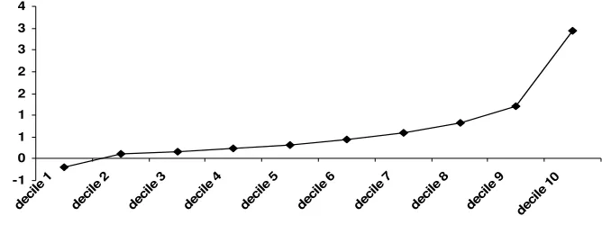
Results of figures 2-9 come from substituting parameters in preceding equation for a year with those parameters for its previous year. In fact, we have substitute price effects for finding a simulated unaffected year. In this point of view, we use a 2-stage Heckman’s method with a special extra equation described before. Figure (2) shows that those policies that affect 1995, decrease averagely an individual enterpriser’s earning who is in the first decile1 as much as 24,680,374 Rials1, and decrease averagely an individual

1

-1 0 1 1 2 2 3 3 4

decile 1

decile 2

decile 3

decile 4

decile 5

deci le 6

deci le 7

deci le 8

deci le 9

dec ile 1

0

M

illio

n

R

ia

ls

enterpriser’s earning who is in the last decile as much as 22,265,804 Rials. We can conclude that the noticed policies cause all enterprisers miss some of their opportunities, but enterprisers with lower income has had a more missing in their opportunities than whom with higher income. In addition, Figure 3 shows that noticed policies make the Lorenz curve have a more unequal situation.

Figure 3: Lorenz curves of enterprisers’ earning in simulated affected year (Tsen95) and simulated unaffected year (Tsen9495) (1995)

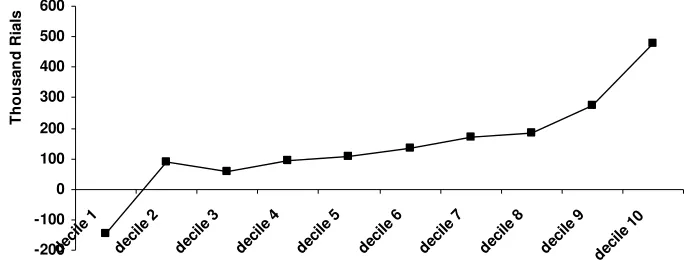
Figure 4: difference between family’s earning per capita in simulated affected year

and simulated unaffected year (1995)

Finally, putting all remuneration effects of wage owners, enterprisers, other income owners, and households’ self employment on income, we find out that 1995’s regime shift affect households incomes like figure 4. the figure shows that an average family in first decile has missed some opportunities in effect of the policy regime shift. On the other hand, an average family in tenth decile has experienced a high income increment which wasn’t affordable in

1

0 50 100 150 200 250 300 350 400 450 500

deci le 1

deci le 2

decil e 3

deci le 4

deci le 5

deci le 6

deci le 7

deci le 8

deci le 9

decile 1 0

Th

ou

s

a

nd

R

ia

ls

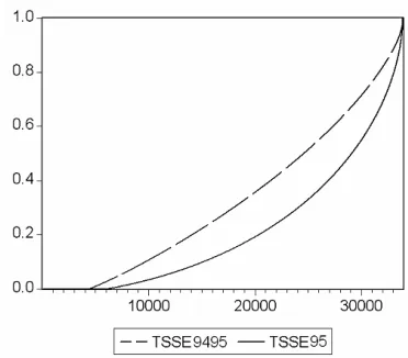
case of omitted policy regime shift. Overall Figure 5 shows that Gini coefficient has increased in effect of the policy regime shift.

Figure 5: Lorenz curves of families’ earning in simulated affected year (Tsse95) and simulated unaffected year (Tsse9495) (1995)

IV.II Year 1998-1999

In 1999, attempts in distributing incomes equally have a successful result in distributing wages, but in other cases government provides unequal effects. In this case, not only Gini Coefficient doesn’t have any increment, but also it shows more equal distribution in 1999, comparing with simulated unaffected year. This proves necessity of using current method to modeling Iranian situation; because in this year, effective policies cause an increase in the highest decile’s earning eight times more than increase in the lowest decile’s earning (Figure 6).

0 400 800 1,200 1,600 2,000

deci le 1

deci le 2

deci le 3

deci le 4

deci le 5

dec ile 6

dec ile 7

deci le 8

deci le 9

deci le 1

0

Thou

s

a

nd R

ia

ls

4,000 4,200 4,400 4,600 4,800 5,000 5,200

deci le 1

deci le 2

deci le 3

deci le 4

dec ile 5

decil e 6

deci le 7

deci le 8

deci le 9

deci le 10

T

hou

s

a

nd R

ia

ls

IV.III Year 2000-2001

In year 2001 there isn’t any determined distributional policy, but lower inflation rate, comparing to previous years, causes an increase in all deciles’ earning (Figure 7).

Figure 7: difference between family’s earning per capita in simulated affected year and simulated unaffected year (2001)

IV.IV Year 2002-2003

Results of micro-simulation year 2003 show an invaluable aspect of current method. After all, Lorenz curve and Gini Coefficient are the same in two simulated situations, but micro-simulation shows an unequal effect of regime shift. However, figure 8 shows that there is not any significant effect of the policy regime shift on enterprisers’ income; moreover, we have found that wage owners have experienced a more equal incomes; but, other income owners have experienced a more unequal incomes.

Figure 8: difference between enterprisers’ earning in simulated affected year and simulated unaffected year (2003)

-200 -100 0 100 200 300 400 500 600

deci le 1

deci le 2

decil e 3

deci le 4

decil e 5

decil e 6

deci le 7

decil e 8

deci le 9

deci le 10

Tho

us

a

n

d R

ia

ls

regime shift; in fact, Lorenz curves are nearly the same. But, one may see in figure 9 that there is a big gap between first decile’s miss and tenth decile‘s gain.

Figure 9: difference between family’s earning per capita in simulated affected year and simulated unaffected year (2003)

V. Conclusions

In this paper, we’ve established a method which computes the effect of policy regime shifts in households’ and individuals’ incomes. This new method helps us to have an acceptable precision in evaluating distributing shape that policy regime shifts have made.

Reference:

[1] A.Alesina, D.Rodrik "Distributive Politics and Economic Growth" The Quarterly Journal of Economics, MIT Press, Vol.109 (2), May 1994, 465-490

[2] C.E.Vélez, J. Leibovich, A. Kúgler, C. Bouillón, and J. Núñez. 2001 “The Reversal of Inequality Trends in Colombia, 1978-1995: A Combination of Persistent and Fluctuating Forces” Mimeo. The World Bank, Washington, DC

[3] D.Bravo, D.Contreras, T.Rau, S.Urzua “Income Distribution in Chile 1990-1998: Learning from Microeconomic Simulation”May 2000

[4] D.Dollar, A.Kraay "Growth Is Good for the Poor" Journal of Economic Growth, Springer, vol. 7(3), September 2002, 195-225

[5] F.Bourguignon, N.Ferreira, N.Lusting “The Microeconomic of income distribution Dynamics In East Asia and Latin America” A co publication of the World Bank and Oxford University Press, September 2004

[6] J.Heckman “Sample selection Bias as a specification error” Econometrica, Vol.74, No. 1, January1979, 153-161

[7] K. J. Forbes "A Reassessment of the Relationship between Inequality and Growth" American Economic Review, American Economic Association, vol. 90(4), September 2000, 869-887