Lancaster University Management School
Working Paper
2005/062
The wage curve revisited: estimates from a UK panel
Geraint Johnes
The Department of Economics Lancaster University Management School
Lancaster LA1 4YX UK
© Geraint Johnes
All rights reserved. Short sections of text, not to exceed two paragraphs, may be quoted without explicit permission,
provided that full acknowledgement is given.
The LUMS Working Papers series can be accessed at http://www.lums.lancs.ac.uk/publications/
THE WAGE CURVE REVISITED: ESTIMATES FROM A UK PANEL
Geraint Johnes
Department of Economics
Lancaster University Management School Lancaster LA1 4YX
United Kingdom
T: +44 1524 594215 F: +44 1524 594244 E: G.Johnes@lancs.ac.uk
October 2005
ABSTRACT
Panel data from the United Kingdom are used to estimate a wage curve that allows simultaneously for time, individual, and spatial effects and which thus finesses the problem of grouped data bias. Once allowance is made for the multilevel and cross-classified nature of the data, estimates of the unemployment elasticity of the wage are seen to be volatile and imprecise.
JEL Classification: J30
Keywords: wage curve, panel data
1. Introduction
Since the pioneering work of Blanchflower and Oswald (1994, 2005), the literature on the wage curve has developed along several lines (Nijkamp and Poot, 2005). Blanchard and Katz (1999) and Black and Fitzroy (2000), for example, have emphasised the importance of using (log) hourly wages (as opposed to annual
earnings) as the dependent variable. Bell et al. (2002) have considered the relationship
between wages, regional and aggregate unemployment, and migration.
The developments of most interest in the present context concern two issues. First, the
original wage curve estimates were subject to grouped data bias (Aitkin et al., 1981;
Moulton, 1986) – since the data used in the analysis were collected at two levels of a hierarchy, namely individual (wages) and region (unemployment), a group effect bias is introduced. This problem was recognised by Blanchflower and Oswald (1994, pp. 168-170) who finessed it by repeating their analysis at the more highly aggregated level using cell means for wage data. While this is a commonly used method, it suffers a major drawback in that it disposes of much individual level data. It also limits the extent to which issues of unobserved heterogeneity across regions can be investigated, although this drawback is mitigated in more recent studies that construct
panels of regions across time (Baltagi et al., 2000; Wu, 2004; Iara and Traistaru,
2004).
The second development is related to the availablility of data. Since the original work on the wage curve was published, many more panel datasets have become available which allow exploration of the importance to the wage curve of unobserved heterogeneity across individuals. These include several German datasets (the German Socio-Economic Panel, studied by Pannenberg and Schearze, 1998, and the Institut fur Arbeitsmarkt und Berufsforschung panel, analysed by Baltagi and Blien, 1998, and by Bellman and Blien, 2001). In other European countries, the European
Community Household Panel has been used by Montuenga et al. (2003) and by
García-Mainar and Montuega-Gómez (2003). And for the US, the National Longitudinal Survey of Youth has provided a wealth of data for analysis by Bratsberg and Turunen (1996) and Turunen (1998).
Several of the studies listed above use the panel data to control for both time and region effects, typically using a fixed effects methodology. Likewise, several studies make reference to grouped data bias as a caveat but do not correct for it. Some others do attempt a correction, but do not arrive at a fully satisfactory fix; for example, Turunen (1998) reports estimates both for equations including fixed effects for region and for those including fixed effects for individuals, but does not include both effects simultaneously. García-Mainar and Montuega-Gómez (2003) are keenly aware of the issues here, and try two methods to fix the problem. The first method, which they deem unsatisfactory, adopts the two-stage approach suggested by Card (1995). Their second method introduces individual intercept shifts by modelling in differences (Arellano and Bond, 1991), which means that much information about the impact of time-invariant cofactors is lost.
on the work of Goldstein (1987, 2003) on multi-level and cross-classified models. The method will be demonstrated using data for the United Kingdom, drawn from the
British Household Panel Survey (BHPS).1 The method also allows analysis of how
the impact of variables other than unemployment on the wage can vary over time. A key finding of the paper is that allowing for the multilevel nature of the data much reduces the precision with which the unemployment elasticity of the wage is estimated, and thereby calls into question much of what we thought we knew about the wage curve.
2. The wage function and data issues
The method used here draws on the literature on multi-level modelling. We have a model where, within a region, measurements on individuals are taken at various points in time. This is not a standard hierarchical model, however, since individuals can move across regions over time. So the focus is on a two level model in which the first level represents occasions, while the second is a cross-classification between individuals and regions (Goldstein, 2003). Occasions (years) can be modelled as fixed effects, while both regions and individuals are associated with random effects. Hence all three sources of unobserved heterogeneity can simultaneously be modelled, with the wage curve taking the form
ln wi(rt) = ai(rt) + fr+ dt + bXi(rt)+ β ln u(rt) + εirt (1)
where wirtdenotes the hourly wage obtained by individual i in region r at time t, urtis
the unemployment rate in region r at time t, and Xirt is a vector of other individual-,
region- and time-specific variables.
The data are taken from the BHPS 1992-2003.2 This is an unbalanced panel of
152640 individuals, of whom 71011 have positive earnings. Of these we have location data for 65601, and this therefore forms the sample on which the analyses are conducted. The loss of more than one half of the observations due to zero earnings is not so much a concern as it might at first appear; since this is a household survey, much non-participation in the labor market is due to respondents’ age. But sample selection biases may remain; we note this as a caveat, but note also that standard solutions to this problem are not presently available for application in the context of a mixed hierarchical and cross-classified model of the type used here.
Unemployment data (from www.nomisweb.co.uk) for October of each year are grafted onto the BHPS using region codes. Ideally one would wish to use more spatially disaggregated data than this, but software constraints preclude this – the modelling of cross-classified data requires us to set up a large number of auxilliary variables. For the same reason we are unable to disaggregate unemployment rates by worker group. Nevertheless, with 11 regions and a panel of length 11, the degrees of freedom on the unemployment variable are comparable with those available in several earlier studies based on panel data.
1
These data were kindly supplied by the UK Data Archive. 2
Control variables used in the analysis include sex (male=1, female=0), age, age squared, marital status (on its own and interacted with sex), number of dependent
children (again on its own and interacted with sex), health status (measured on a 5
point scale from excellent=1 to poor=5), union membership (member=1,
non-member=0) and binary variables indicating the highest educational qualification.
These vary from higher degree (hidegree) through bachelor’s degree (degree), nursing
qualification (nursingq), upper secondary school qualifications (alevels), lower
secondary school qualifications (olevels) and other qualifications (othqual).
3. Results
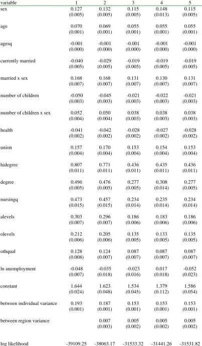
Results, obtained using MLwiN 2.02, are reported in Table 1; these allow fully, both in estimation of coefficients and standard errors, for the grouped and cross-classified nature of the data. In column 1 we report an equation in which there are fixed effects for years and random effects for individuals, but where no allowance is made for a region effect, so that the group nature of the unemployment variable is not accommodated. It is readily seen that this specification yields a fairly conventional wage curve; the estimated unemployment elasticity of the wage is, in absolute terms, somewhat lower than the conventional value of –0.1 suggested by Blanchflower and Oswald’s ‘empirical law’, but it is negative and very highly significant. The values of the other coefficients all accord with the conventional wisdom. Some of the explanatory variables, in particular those referring to marital status and childrearing, are potentially endogenous; excluding them from the analysis makes no substantive difference to the coefficients on the remaining variables.
Column 2 reports the results obtained once equation (1) is estimated, that is with individual and regional random effects and time fixed effects. While most of the estimated coefficients are robust to this change, the absolute value of the estimate of the unemployment elasticity of the wage drops, and, having previously been very highly significant, it is now significant only at levels in excess of 5 per cent. This finding echoes those of Bratsberg and Turunen (1996) and Turunen (1998).
In column 3, we add dummies for (9) industries and (9) occupations. As might be expected, this reduces the magnitude on the coefficients on the education variables; it also reduces further both the estimate of the unemployment elasticity of the wage and its significance.
Column 4 reports the outcome when the model is augmented further by a full set of interaction terms between years and (i) sex, (ii) degree, and (iii) logged unemployment. In each case, 1992 is the omitted interaction. These fixed effects are not reported in full for reasons of space, but the main findings may be summarised here. The magnitude of the male wage premium declined over the period; while in 1992 it amounted to 0.148, by 2003 it had declined to 0.097; the slope dummies are consistently significantly negative from 1998 on. Likewise the wage premium attached to degree-level educational qualifications (over and above no qualifications,
and controlling, inter alia, for occupation) declined from 0.308 in 1992 to 0.260 in
in educational level would be rare and changes in sex (probably) nonexistent. Finally, and of most interest in the present context, the unemployment elasticity of the wage
varied from a high of +0.017 in 1992 to a low of –0.054 in 1995.3 This last finding
reinforces observations made by Turunen (1998) about the instability of the wage curve over time.
Some authors have raised concerns about the possible endogeneity of unemployment in wage curves models of the type estimated here (see, for example, Baltagi and Blien, 1998). To check for this, we rerun the model reported in column 3, this time instrumenting (on the lag of logged unemployment) for the unemployment variable. The effect of this is to increase somewhat the absolute value of the estimate of the unemployment elasticity of the wage, but the estimate remains insignificant at the 5 per cent level.
While it is not possible to estimate a wage curve for the whole of the UK using highly disaggregated unemployment data, it is possible to study smaller labor market areas if we restrict the sample to a single region, and then disaggregate the unemployment measure to the level of the local authority district. If this is done, similar findings to those reported above obtain. For example, the coefficients on logged unemployment that obtain in the London and South East regions corresponding to columns 1 and 2 of Table 1 are –0.017 (with a standard error of 0.007) and –0.027 (with a standard error of 0.019) respectively. The wage curve appears to be a context in which grouped data bias really matters.
4. Conclusions
The results reported above indicate that, once allowance is simultaneously made for unobserved heterogeneity at both the individual and region level and the grouped nature of the data are accommodated, the unemployment elasticity of the wage is both volatile and, in some specifications at least, imprecisely determined. The estimates reported here suggest that, while a wage curve appears to exist for the whole of the UK in some periods, its shape does not generally accord with any general ‘empirical law’. Further research using panels for other countries is clearly warranted.
References
Aitkin, Murray, Anderson, Dorothy and Hinde, John, 1981. Statistical modelling of data on teaching styles, Journal of the Royal Statistical Society A 144, 419-461.
Arellano, Manuel and Bond, Stephen, 1991. Some tests of specification for panel data: Monte Carlo evidence and an application to employment equations. Review of Economic Studies 58, 277-297.
Baltagi, Badi H. and Blien, Uwe, 1998. The German wage curve: evidence from the IAB employment sample. Economics Letters 61, 135-142.
3
Baltagi, Badi H., Blien, Uwe and Wolf, Katja, 2000. The East German wage curve 1993-1998. Economics Letters 69, 25-31.
Bell, Brian, Nickell, Stephen J. and Quintini, Glenda, 2002. Wage equations, wage curves and all that. Labour Economics 9, 341-360.
Bellman, Lutz and Blien, Uwe, 2001. Wage curve analyses of establishment data from Western Germany. Industrial and Labor Relations Review 54, 851-863.
Black, Angela and Fitzroy, Felix, 2000. Earnings curves and wage curves. Scottish Journal of Political Economy 47, 471-486.
Blanchflower, David G. and Oswald, Andrew J., 1994. The wage curve, Cambridge MA: MIT Press.
Blanchflower, David G. and Oswald, Andrew J., 2005. The wage curve reloaded. NBER Working Paper 11338.
Bratsberg, Bernt and Turunen, Jarkko, 1996. Wage curve evidence from panel data. Economics Letters 51, 345-353.
Card, David, 1995. The wage curve: a review. Journal of Economic Literature 33, 785-799.
Goldstein, Harvey, 1987. Multilevel covariance component models. Biometrika 74, 430-431.
Goldstein, Harvey, 2003. Multilevel statistical models (third edition), London: Hodder Arnold.
Iara, Anna and Traistaru, Iulia, 2004. How flexible are wages in EU accession countries? Labour Economics 11, 431-450.
Montuenga, Víctor, García, Inmaculada and Fernández, Melchor, 2003. Wage flexibility: evidence from five EU countries based on the wage curve. Economics Letters 78, 169-174.
García-Mainar, Inmaculada and Montuenga-Gómez, Víctor M., 2003. The Spanish wage curve 1994-1996. Regional Studies 37, 929-945.
Moulton, Brent R., 1986. Random group effects and the precision of regression estimates. Journal of Econometrics 32, 385-397.
Nijkamp, Peter and Poot, Jacques, 2005 The last word on the wage curve? Journal of Economic Surveys 19, 421-450.
Pannenberg, Markus and Schwarze, Johannes, 1998. Labor market slack and the wage curve. Economics Letters 58, 351-354.
Tutunen, Jarkko, 1998. Disaggregated wage curves in the United States: evidence from panel data of young workers. Applied Economics 30, 1665-1677.
Table 1 Regression results: dependent variable is the log of the hourly wage
variable 1 2 3 4 5
sex 0.127 0.132 0.115 0.148 0.115
(0.005) (0.005) (0.005) (0.013) (0.005)
age 0.070 0.069 0.055 0.055 0.055
(0.001) (0.001) (0.001) (0.001) (0.001)
agesq -0.001 -0.001 -0.001 -0.001 -0.001
(0.000) (0.000) (0.000) (0.000) (0.000)
currently married -0.040 -0.029 -0.019 -0.019 -0.019 (0.005) (0.005) (0.005) (0.005) (0.005)
married x sex 0.168 0.168 0.131 0.130 0.131
(0.007) (0.007) (0.007) (0.007) (0.007)
number of children -0.050 -0.045 -0.021 -0.022 -0.021 (0.003) (0.003) (0.003) (0.003) (0.003)
number of children x sex 0.052 0.050 0.038 0.038 0.038 (0.004) (0.004) (0.003) (0.003) (0.003)
health -0.041 -0.042 -0.028 -0.027 -0.028
(0.002) (0.002) (0.002) (0.002) (0.002)
union 0.157 0.170 0.153 0.154 0.153
(0.004) (0.004) (0.004) (0.004) (0.004)
hidegree 0.807 0.771 0.436 0.435 0.436
(0.011) (0.011) (0.011) (0.011) (0.011)
degree 0.496 0.476 0.277 0.308 0.277
(0.005) (0.005) (0.005) (0.014) (0.005)
nursingq 0.473 0.457 0.234 0.235 0.234
(0.015) (0.015) (0.014) (0.014) (0.014)
alevels 0.303 0.296 0.186 0.183 0.186
(0.007) (0.007) (0.006) (0.006) (0.006)
olevels 0.212 0.205 0.135 0.133 0.135
(0.006) (0.006) (0.005) (0.005) (0.005)
othqual 0.128 0.124 0.087 0.087 0.087
(0.008) (0.007) (0.007) (0.007) (0.007)
ln unemployment -0.048 -0.035 -0.023 0.017 -0.052
(0.007) (0.018) (0.016) (0.018) (0.023)
constant 1.644 1.623 1.534 1.379 1.586
(0.024) (0.048) (0.045) (0.112) (0.054)
between individual variance 0.193 0.187 0.153 0.153 0.153 (0.001) (0.001) (0.001) (0.001) (0.001)
between region variance 0.007 0.005 0.005 0.005
(0.003) (0.002) (0.002) (0.002)