Munich Personal RePEc Archive
Simulated maximum likelihood for
general stochastic volatility models: a
change of variable approach
Kleppe, Tore Selland and Skaug, Hans J.
10 July 2008
Online at
https://mpra.ub.uni-muenchen.de/12022/
Simulated maximum likelihood for general
stochastic volatility models: a change of variable
approach
Tore Selland Kleppe
∗and Hans Julius Skaug
†July 10, 2008
Abstract
Maximum likelihood has proved to be a valuable tool for fitting the log-normal stochastic volatility model to financial returns time series. Us-ing a sequential change of variable framework, we are able to cast more general stochastic volatility models into a form appropriate for importance samplers based on the Laplace approximation. We apply the methodol-ogy to two example models, showing that efficient importance samplers can be constructed even for highly non-Gaussian latent processes such as square-root diffusions.
Keywords: Change of Variable, Heston Model, Laplace Importance
Sam-pler, Simulated Maximum Likelihood, Stochastic Volatility
∗Department of Mathematics, University of Bergen, Johannes Brunsgate 12, 5008 Bergen, Norway, Email: [email protected] (Corresponding author)
1
Introduction
During the last two decades, a vast literature on fitting stochastic volatility
(SV) models to price return data has emerged. Parameter estimation in such
models is made difficult by the presence of a latent volatility process. The
recent approaches follow essentially two lines of attack for integrating out the
volatility: simulated maximum likelihood (SML) (e.g. Danielsson and Richard
(1993); Danielsson (1994); Shepard and Pitt (1997); Sandmann and Koopman
(1998); Liesenfeld and Richard (2003, 2006); Durham (2006, 2007); Richard
and Zhang (2007)) and Markov chain Monte Carlo (MCMC) (e.g. Omori et al.
(2007) and refrences therein). In this paper we seek to extend the class of SV
models that can be efficiently fit using SML, and hence to provide access to the
maximum likelihood toolbox.
Earlier SML approaches are mainly focused around extensions of the
discrete-time log-normal SV model (Taylor, 1982)
Xt=
p
Vtηt, t= 1, . . . , n (1)
Vt=σX2 exp(Ut) (2)
Ut=φUt−1+σZt, t= 2, ..., n (3)
U1=
σ
p
1−φ2Z1 (4)
where (φ, σ, σX) are parameters and (ηt, Zt), t = 1, . . . , n are i.i.d. standard
Gaussian variates. Here, Xt is the process of price log-returns and Vt is the
volatility process. The Gaussian AR(1) processUtis typically highly
autocorre-lated, with a small transition varianceσ2. The success of Laplace approximation
(applied toU= [U1, . . . , Un]′), and the associated SML, may be traced back to
the fact that the conditional probability density function (PDF) ofU givenX
A large number of other SV models, in particular in continuous-time, have
been proposed in literature (e.g. Nelson (1990); Heston (1993);
Barndorff-Nielsen and Shephard (2001); Durbin and Koopman (2001); Jones (2003); Barndorff-Nielsen
and Shephard (2003)) and are typically specified as a bi-variate stochastic
pro-cess{(Xt, Vt)}whereVt>0 is a Markov process andtindexes either
continuousor discretetime. Inspired by the high accuracy of Laplacebased SML fcontinuousor (1
-4) in Ut, we introduce a Gaussian white noise process Zt and re-specify the
original model (Xt, Vt) as (Xt, Zt) so that the marginal distribution (and hence
the likelihood) ofXtsampled at discrete timesXis equal in both models.
Ap-plication of Laplace importance samplers in the correspondingZyield a rapidly
converging approximation of the likelihood function, and for a fixed number of
importance samples, this approximate likelihood function can be maximized to
obtain parameter estimates and approximate test statistics.
A prerequisite for this approach is that the PDF of (X,V) at a collection of
time points 1, . . . , nmay be written on the form
pX,V(x,v) =pX1,V1(x1, v1)
n
Y
i=2
pXi,Vi|Vi−1(xi, vi|vi−1) (5)
and that the transition probability density (TPD)pXi,Vi|Vi−1(xi, vi|vi−1) can be
evaluated efficiently. For continuous-time models, the observations need not to
be at equidistant times as long as the TPDs can be calculated accordingly.
The rest of the paper is laid out as follows. Section 2 is devoted to an
outline of the proposed change of variable methodology, and we illustrate some
important features through simple examples. Some issues of implementation
are also discussed. In section 3 we illustrate the methodology through fitting
two example models to the classic Dollar/Pound dataset (Harvey et al., 1994).
The first model considered is the log-normal model (1 - 4), but we depart from
model is a semi-discrete version of the Heston model (Heston, 1993), where
the volatility process follows a continuous-time square-root diffusion. Finally,
section 4 provides some discussion.
2
Methodology
In this section, we outline the proposed methodology to transform a general
stochastic volatility model likelihood problem into a form suitable for Laplace
importance sampler analysis. First, we review some basic facts concerning
vari-able transforms and the Laplace approximation. Then we motivate and state
the general sequential change of variable map that constitutes the core of this
work. Finally we consider implementation issues.
2.1
Changes of variables and Laplace approximations
At the core of any textbook in multivariate calculus is the change of variable
formula for integrals
Z
Rn
f(v)dv=
Z
Rn
f(ψ(z))|∇ψ(z)|dz, (6)
where ψ:Rn →Rn and one-to-one, and |∇ψ(z)| is the Jacobian determinant of ψ (Sydsæter et al., 1999). When n is large, the Laplace approximation
(Barndorff-Nielsen and Cox, 1989) and related importance samplers (Kuk, 1999;
Skaug, 2002) are the workhorses for approximating integrals on this form. The
Laplace approximation is given as
Z
Rn
f(v)dv≃f(ˆv) (2π)
n/2
p
where |∇2g(ˆv)| is the determinant of the Hessian of g(v) at the minimizer
ˆ
v. It is easily verified that the Laplace approximation is nothing more than
approximating the integrand with an un-normalizedN(ˆv,
∇2g(ˆv)−1
) density
and calculating the exact integral over the approximate integrand. We refer to
this Gaussian PDF as the Laplace approximating density (LAD). In itself, the
Laplace approximation is fairly accurate over a large class of integrals, but the
fixed accuracy is a drawback. To work around this, we use Laplace importance
samplers (LIS)
ILIS=
1
m
m
X
i=1
f(vi)
pLAD(vi)
withvi, i= 1, . . . , miid sampled from the LAD. Provided thatvar(ILIS)<∞,
ILIS converges strongly, asm→ ∞, to the exact value of the integral. We shall
use the terms Laplace approximation and Laplace importance samplers more or
less interchangeably.
Combining (6) with the LIS sets the stage for the rest of the discussion
here. Since the change of variable mapψis to our disposition, we hope that by
approximating the right hand side of (6) with a LIS, the Monte Carlo variance
can be reduced significantly compared to applying a LIS to the left hand side.
Some properties of the Laplace approximation deserve mentioning here. The
Laplace approximation is exact when the integrand is an un-normalized
Gaus-sian density. As noted in Butler (2007), the Laplace approximation is invariant
under affine changes of variable in the original integral. Both of these properties
extends trivially to the LIS and points out some directions as how to chooseψ.
An affineψwill not improve anything, and the right hand side integrand in (6)
should be close to an un-normalized Gaussian density.
If the Laplace approximation is applied to a marginalization integral in a
latent variable model, say (X,V) withVlatent, then the mode ˆvis the empirical
likelihood estimate (Carlin and Louis, 1996). In the context of SV models, this
may be applied to smooth and filter the volatility process.
2.2
A toy example
Consider the following one-dimensional example. Let X ∼ N(0, V) and V ∼
lognormal(0, σ). This may be thought of as a special case of the SV model (1
- 4) with only one observation. To calculate the PDF ofX marginally, i.e. the
likelihood, we need to integrate out the latentV:
pX(x) =
Z
pX|V(x|v)pV(v)dv
=
Z
R
1 √
2πvexp(− x2 2v)
1
vσ√2πexp(−
(log(v))2
2σ2 )1{v>0}(v)dv, (8)
where 1denotes the indicator function. Now, consider the change of variable
mapv=ψ(z) =F−1(Φ(z)) = exp(σz), where Φ denotes the standard Gaussian cumulative distribution function (CDF) andF is the CDF associated withpV.
Simple manipulations yield that the integral (8) may be rewritten as
pX(x) =
Z
R
1
p
2πexp(σz)exp(−
x2 2 exp(σz))
1 √
2πexp(− z2
2)dz. (9)
Simple probabilistic arguments suggest that the variance of LISs applied to both
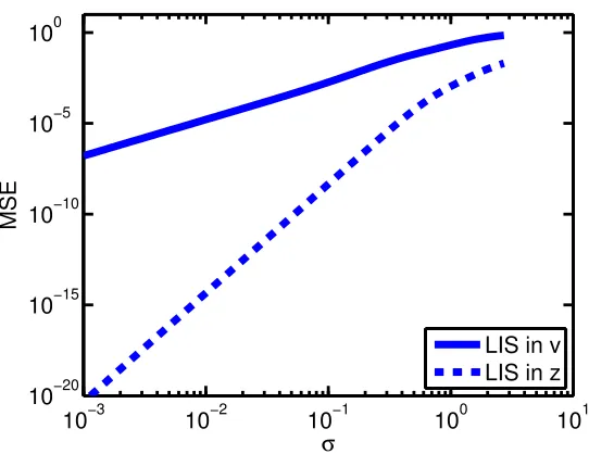
integrals converges to 0 asσ→0. However, the order of magnitude in the mean
square error (MSE) of LISs applied to the two differ significantly as depicted in
Figure 1. There are several partial explanations to this. First, since the integral
(8) is taken over the positive half line, there is always positive probability that
samples from the LAD hit outside the support, slowing down convergence of the
importance sampler. By the simple change of variable, this is fixed for in (9).
10−3 10−2 10−1 100 101 10−20
10−15 10−10 10−5 100
σ
MSE
[image:8.612.171.442.120.329.2]LIS in v LIS in z
Figure 1: Monte Carlo estimates of the mean square error (MSE) in the cal-culation of pX in section 2.2 using LISs withm = 32 importance samples for
different values of the parameter σ. The MSEs are estimated over 1000 runs of the importance samplers for each value ofσ. “LIS in v” refers to the LIS applied to (8) whereas “LIS in z” refers to a LIS applied to (9).
which (9) approaches an un-normalized Gaussian PDF is much higher, yielding
a faster converging importance sampler.
All previous authors who have applied SML to the SV model (1 - 4) have
applied an approximation to an integral corresponding to (9), and the above
example may thus seem somewhat artificial. However, more general SV models
are naturally cast in terms of the non-Gaussian variableV, leading to an integral
similar to (8). Maps on the formψ(z) =F−1(Φ(z)) constitute the backbone in our methodology for transforming integrals from the form (8) to (9).
Another change of variable in (9), sayu=σz, would have brought us closer
to the practice of integrating in theU variables in the log-normal SV model.
This illustrates that it irrelevant whether the “small number” representing the
un-derlying Gaussian as the Laplace methodology is invariant under linear variable
changes. Throughout this paper, we will for simplicity, leave it inψand let the
“driving” vectorZbe standard Gaussian white noise.
2.3
A sequential change of variable framework
The map introduced in the previous example generalizes naturally to the
se-quential change of variable framework
v=ψ(z) =
ψ1(z)
ψ2(z) .. .
ψn−1(z)
ψn(z)
=
F1−1(Φ(z1))
F2−1(Φ(z2), v1) .. .
Fn−−11(Φ(zn−1), vn−2)
F−1
n (Φ(zn), vn−1)
. (10)
For now, we let theFis be absolutely continuous CDFs in their first argument.
Specific choices are discussed shortly. It is easily verified, by an induction
argu-ment forward in time, that (10) is a one-to-one mapping.
The strict one-step-backward dependence is introduced to mimic the Markov
structure of (X,V) and has the pleasant feature of a triangular Jacobian. This
last fact leads to a particularly simple formula for the log-Jacobian determinant:
log|∇ψ(z)|=−n2 log(2π)−
n X i=1 1 2z 2
i −logp1(v1(z))−
n
X
i=2
logpi(vi(z), vi−1(z)),
the general modified negative log-integrand inz.
g∗(z) =n
2log(2π)+ 1 2
n
X
i=1
zi2−[logpX1|V1(x1|v1(z))+logpV1(v1(z))−logp1(v1(z))]
−
n
X
i=2
logpXi|Vi(xi|vi(z)) + logpVi|Vi−1(vi(z)|vi−1(z))−logpi(vi(z), vi−1(z))
.
(11)
2.4
Choices of
F
iIn this work, we consider two specific choices of theFis that are rather apparent
given (11). These are chosen under the constraints that they are easy to evaluate
and invert, and that they apply to a broad class of models.
If we take Fi, i = 2, . . . , n to be the CDFs of Vi|Vi−1, and let F1 be the limiting CDF ofVt, we get a sequential change of variable map which we will
denoteψ(1). Under this formulation, the negative log-integrand (11) takes the
form:
g∗
(1)(z) =
n
2 log(2π) + 1 2 n X i=1 z2 i − n X i=1
logpXi|Vi(xi|vi(z))
= n
2log(2π) + 1 2
n
X
i=1
z2i − n
X
i=1
Mi(1)(vi(z)). (12)
Typically, if the volatility process has small variance relative to 1,v(z) will vary
slowly and the standard Gaussian part will dominate the total variation ofg∗
(1).
Underψ(1), the distributions ofVandψ(1)(Z) are equal, and we may interpret
the methodology as simply adding a new level in the hierarchical representation
of the SV model.
We denote by ψ(2) the sequential change of variable map when F
i, i =
2, . . . , n are taken to be the CDFs of Vi|Vi−1, Xi and F1 to be the CDF of
negative log-integrand has the form
g∗(2)(z) = n
2 log(2π) + 1 2
n
X
i=1
zi2− n
X
i=2
logpXi|Vi−1(xi|vi−1(z))−pX1(x1)
= n
2log(2π) + 1 2
n
X
i=1
zi2− n
X
i=2
Mi(2)(vi−1(z))−M1(2).
It is reasonable to assume, and we shall see this in the examples, that ψ(2)
should lead to faster convergence of the LIS since M(2) depends more weakly
onzthan doesM(1). The drawback is that theψ(2) formulation typically leads
to non-standard CDFs that need to be evaluated using numerical integration
techniques.
By construction, choosing one of these maps resolves the issues concerning
the joint support of the latent process. This is of particular importance in
models where the support ofVi|Vi−1depends onVi−1, such as in the exponential AR(1) process proposed by Nielsen and Shephard (2003) or the gamma AR(1)
processes proposed by Durbin and Koopman (2001).
A few more points deserve mentioning here. In both formulations, it is not
essential to have an explicit limiting distribution for the volatility process. This
can be worked around by starting the latent process in some fixed point at some
time prior to where we have data, and then let it be integrated out. Missing
data can be handled equally well in this manner. Moreover, the explicit splitting
of the PDFs into transition and observation parts seen in (11) is not strictly
2.5
A simple explicit example
Consider a modified version of the SV model proposed in Nielsen and Shephard
(2003),
Xt=
p
Vt+γ ηt, t= 1, . . . , n
Vt=φVt−1+λεt, t= 2, . . . , n
V1=
λ
1−φε1,
whereηt, t= 1, . . . , nare iid standard Gaussian,εt, t= 1, . . . , nare i.i.d. exp(1)
andλ, γ >0,φ∈[0,1) are parameters. For simplicity, we have chosen the start
condition so that it matches the mean of the limiting distribution. Underψ(1),
this model admits an explicit sequential change of variable map given by the
recursion
v1=−
λ
1−φlog(1−Φ(z1))
vi=φvi−1−λlog(1−Φ(zi)), i= 2, . . . , n
and it is easy to verify that the gradient and Hessian ofg∗
(1) are on the form
h
∇g(1)∗ (z)
i
i=zi+O(λ)
h
∇2g∗(1)(z)
i
ij =
1 +O(λ) ifi=j
O(λ2) otherwise
for fixed values ofφ,γand small values ofλ. Moreover all the higher derivatives
are at least O(λ) as one would expect. This suggests that for small λ, the
transition standard deviation, a high degree of accuracy could be expected when
process, i.e. Xtis i.i.d. N(0, γ), is smooth both theoretically and numerically.
2.6
Derivative calculations and implementation issues
For the proposed methodology to be applicable, it is essential that the first and
second order derivative arrays of the negative modified log-integrandg∗(z) can
be evaluated efficiently. The sparsity pattern in the Hessian matrix seen in the
classical treatment of the log-normal SV model (1 - 4) is in general lost with the
introduction of the change of variable map. Still, we can find efficient methods
for calculating derivatives using a combination of forward and backward mode
algorithmic differentiation (AD) techniques (Griewank, 2000).
In the current work, the derivative calculations are done in two phases based
on the local preaccumulation principle in Griewank (2000). First, we calculateg∗
forward in time, and concurrently, calculate and store the first and second order
partial derivatives ofMi andψi. Since the dependence structure is completely
given by (10), backward accumulation of the gradient and Hessian can be done
secondly in only O(n) and O(n2) operations respectively, with only a small
multiple ofnextra memory required. Note that the computational cost of the
determinant evaluation in (7) is O(n3), and hence the cost of the derivative
calculation will be neglectible whenngets large. We use the AD tool Tapenade
(Hascoët and Pascual, 2004) to generate multi-directional forward mode code
for the derivatives of ψi andMi, whereas the backward accumulation schemes
have been hand coded. This balance between backward and forward AD yields
a fast and memory-efficient code, which is easily adapted to new models.
All non-trivial one-dimensional integrals are evaluated using the integrals of
Chebyshev interpolating polynomials (Press et al., 1992) to obtain fast repeated
evaluation of the approximate CDFs and smooth code. The optimization
(2006). First a BFGS quasi-Newton solver (Nocedal and Wright, 1999), then
a full Newton solver (Nocedal and Wright, 1999). The BFGS solver provide
stability over a large part of the parameter space, whereas the Newton solver
lets us solve the inner problem to machine precision to keep the simulated
like-lihood function smooth. Common random numbers in the importance samplers
is another remedy applied for keeping the likelihood approximation smooth. For
each of the i.i.d. standard Gaussian vectors used to simulate from the LAD, we
use four antithetics to balance for location and scale (Durbin and Koopman,
2001).
3
Application to real data
To illustrate the proposed methodology, we fit two models to the classic data set
of log-returns of the Dollar/Pound exchange rate from 01/10/1981 to 28/06/1985
(Harvey et al., 1994). The data consist of a total ofn= 945 log-return
obser-vations.
The first model is the log-normal SV model (1 - 4), but with the latent
pro-cess taken to beVtin (2), i.e. the process with log-normal marginals. This
ex-ample is included for two reasons. First, it shows that the current methodology
gives accurate results compared to highly model-specific methods in previous
work. Secondly, it provides a reference for comparison between the two
mod-els. The second example considers a simplified semi-discretized version of the
Heston model (Heston, 1993) where the volatility process follows a square-root
diffusion. Simulated likelihood analysis under such a volatility process is, to our
knowledge, new.
In both examples, we usem= 128 samples from the LAD, based on 32 i.i.d.
3.1
The log-normal SV model
The log-normal SV model fitted to the classic Dollar/Pound data have been
thoroughly analyzed by Harvey et al. (1994); Shepard and Pitt (1997); Durbin
and Koopman (2001); Liesenfeld and Richard (2006) using simulated likelihood
and MCMC methods. Common for the simulated likelihood approaches is that
the latent process is taken to be the Gaussian AR(1) process (3), thus yielding
a near-Gaussian integrand suitable for straight forward LIS. Here, we disregard
the Gaussian processUt, and apply the methodology directly toVt, so that our
ψ(1) map is equivalent to the approach taken by previous authors.
The setup is as follows. We first estimate the parameters for the
Dol-lar/Pound data 100 times with different seeds in the importance sampler. This
is done to assess the convergence of the importance samplers for the chosen value
ofm. For a single simulation (seed) in theψ(2) formulation, the function
mini-mizer failed to meet the convergence criterion, and this simulation replica was
ignored. We take the mean of the parameter estimates (column 1 in Table 1) to
be our “best estimates”. Then we conduct a parametric bootstrap experiment
using 100 simulated data sets each of lengthn= 945, with the mean
parame-ter estimates as “true” parameparame-ters. Resulting estimates of bias, variance and
correlation are summarized in Table 1.
The most prominent feature of this analysis is that the Monte Carlo standard
errors forψ(2)are reduced by a factor≈4 relative to those ofψ(1)using the same
number of importance samples. This supports the hypothesis thatψ(2)takes the
modified negative log-integrand (11) closer to a quadratic form. The parameter
estimates are very much in accordance with those presented in previous work,
e.g. (φ, σ, σX) = (0.9731, 0.1726, 0.6338) in Durbin and Koopman (2001). The
parametric bootstrap based standard errors and covariance matrices are also
Monte Carlo Parametric bootstrap MC Mean MC S.E. Bias S.E. Correlations
φ σ σX
ψ(1)
φ 0.9742 0.0012 0.0095 0.0176 1 -0.5975 0.0403
σ 0.1709 0.0041 -0.0101 0.0344 1 -0.1279
σX 0.6317 0.0014 -0.0061 0.0709 1
l -918.662 0.2554
ψ(2)
φ 0.9741 0.0003 0.0095 0.0177 1 -0.5963 0.0391
σ 0.1715 0.0007 -0.0105 0.0344 1 -0.1263
σX 0.6315 0.0003 -0.0061 0.0708 1
[image:16.612.147.476.454.504.2]l -918.648 0.0657
Table 1: Parameter estimates for the log-normal SV model fit to the Dol-lar/Pound data. The first two columns show the mean and standard deviation calculated across the maximum likelihood estimations using different seeds in the importance sampler. l denotes the negative log-likelihood approximation. The remaining columns show the results of the parametric bootstrap experi-ment.
3.2
A semi-discrete version of the Heston model
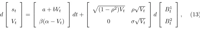
The Heston model (Heston, 1993) in a fairly general form may be written as the
stochastic differential equation (Aït-Sahalia and Kimmel, 2007)
d st Vt =
a+bVt
β(α−Vt)
dt+
p
(1−ρ2)V
t ρ√Vt
0 σ√Vt
d B1 t B2 t
, (13)
wherestis the log-price and (Bt1, Bt2) are independent standard Brownian
mo-tions. To be consistent with log-normal SV model we assume that observations
are on a daily time scale, and simplify the model (to keep the exposition clear
without too many technicalities) using Euler discreteization with time-step 1 on
the price process and seta=b=ρ= 0. Then
st+1=st+
p
Vtηt =⇒ Xt=st+1−st=
p
where ηt are i.i.d. N(0,1) shocks, Xt is the process of log-returns and Vt as
in (13). These simplifications may be interpreted as observing the
continuous-time volatility process with multiplicative noise at a collection of discrete continuous-times
t= 1, . . . , n.
The volatility process is strictly positive when 2αβ > σ2and forβ >0, the
process is stationary and has the property of mean reversion towards the long
run meanα. The TPD can be shown to be a scaled non-central χ2 (Cox et al.,
1985) and the marginal distribution is a gamma. See Cox et al. (1985) for a
complete characterization of these properties.
In all of the computations, we use a re-normalized saddlepoint approximation
(Butler, 2007) to the non-centralχ2 density to obtain fast, stable and smooth
evaluation over the whole parameter space. The setup is as in the previous
example with 100 maximum likelihood estimations of the Dollar/Pound data
set using different seeds and 100 parametric bootstrap estimations. In theψ(2)
computations, two runs for both Monte Carlo and parametric bootstrap failed
to converge, and were consequently ignored.
The results are given in Table 2, and again we see that an approximate
four-fold decrease in Monte Carlo error when switching fromψ(1) to ψ(2).
3.3
Comparison and diagnostics
Since the price return process in both models is linked to the volatility process
in the same manner, we may directly compare the estimated volatility processes.
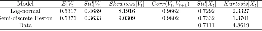
A brief numeric summary of the volatility processes and resulting properties of
the price return data are given in Table 3. We see that the volatility process
of the semi-discrete Heston model is estimated to have a smaller marginal
stan-dard deviation and higher temporal correlation than the log-normal counterpart.
Monte Carlo Parametric bootstrap MC Mean MC S.E. Bias S.E. Correlations
α β σ
ψ(1)
α 0.5425 0.0225 -0.0328 0.1154 1 -0.2206 0.0615
β 0.0194 0.0046 -0.0060 0.0120 1 0.7525
σ 0.0959 0.0079 -0.0043 0.0209 1
l -920.322 1.0006
ψ(2)
α 0.5376 0.0049 -0.0408 0.1197 1 -0.2667 -0.0119
β 0.0200 0.0011 -0.0064 0.0126 1 0.7674
σ 0.0991 0.0025 -0.0055 0.0230 1
[image:18.612.134.449.123.283.2]l -920.148 0.2362
Table 2: Parameter estimates and parametric bootstrap summary for the semi-discrete Heston model. See the caption of Table 1 for details.
Model E[Vt] Std[Vt] Skewness[Vt] Corr(Vt, Vt+1) Std[Xt] Kurtosis[Xt]
Log-normal 0.5317 0.4689 8.1916 0.9662 0.7292 2.3327 Semi-discrete Heston 0.5376 0.3633 9.0309 0.9802 0.7332 1.3701
Data 0.7111 4.8619
Table 3: Properties of the two volatility process and the resulting log-returns, for the Dollar/Pound data. Moments are evaluated under a stationary assumption on{Vt}and for parameter estimates based onψ(2).
in Figure 2. It is immediate that the AIC based on the estimated likelihood
values suggest that the log-normal SV model is the better model for these data
as the two models have the same number of parameters. Discrepancy between
the estimated and empirical standard deviations and kurtosis of the observed
data presented in Table 3 further supports this.
4
Discussion
In the current paper, we have proposed a general methodology for casting
non-Gaussian volatility problems into a form suitable for LIS-approximation of the
likelihood function. The results we have presented suggest that models with a
[image:18.612.143.580.327.379.2]0 200 400 600 800 1000 −4
[image:19.612.179.430.262.459.2]−2 0 2 4 6
We have gone to some length to keep the proposed framework fairly general,
so there is clearly scope for tuning for specific models. One such example, given
that the specific volatility process limiting density has the same support as
the transition density, would be to take theFis to be the CDFs ofVi|Xi. This
formulation has the fortunate property of preserving the tri-diagonal form of the
Hessian, but the performance of the LIS is dependent on the mixing properties
of the volatility process.
For a specific model, it is natural to ask which of the sequential change of
variable maps is preferable from a computational perspective. Judging from the
two example models considered here, one need about a 16-fold increase in the
number of importance samples to obtain the same precision forψ(1) as for that
of ψ(2) (column 2 in Tables 1 and 2). For models that have an explicit ψ(1),
this may still be preferable, as most of the computational burden in the current
implementation lies in the evaluation and inversion of theFis. If the sequential
change of variable map cannot be made explicit, one is almost always certain
to be better off withψ(2).
The idea of changing the integration variables is not new (Mackay, 1998).
Still, it is an area that has received very little attention in the latent variable
maximum likelihood literature, considering its huge potential.
The examples presented in this work do by no means deplete the potential of
these methods. There are no immediate reasons why models displaying
asym-metries and other real-world properties of financial time series should not work,
as long as the corresponding TPDs may be computed efficiently. In the
con-text of continuous-time models, the TPD-expansions of Aït-Sahalia and Kimmel
(2007) may prove valuable, but this is still a question that will require further
References
Aït-Sahalia, Y. and R. Kimmel (2007). Maximum likelihood estimation of
stochastic volatility models. Journal of Financial Economics 134, 507–551.
Barndorff-Nielsen, O. E. and D. R. Cox (1989). Asymptotic techniques for use
in statistics. Chapman & Hall.
Barndorff-Nielsen, O. E. and N. Shephard (2001). Non-gaussian
ornstein-uhlenbeck-based models and some of their uses in financial economics.Journal
of the Royal Statistical Society. Series B (Statistical Methodology) 63, 167–
241.
Butler, R. (2007). Saddlepoint Approximations with Applications. Cambridge
University Press.
Carlin, B. P. and T. A. Louis (1996). Bayes and Empirical Bayes Methods for
Data Analysis. Chapman & Hall.
Cox, J. C., J. E. Ingersoll, and S. A. Ross (1985). A theory of the term structure
of interest rates. Econometrica 53(2), 385–407.
Danielsson, J. (1994). Stochastic volatility in asset prices: Estimation with
simulated maximum likelihood. Journal of Econometrics 64, 375–400.
Danielsson, J. and J. F. Richard (1993). Accelerated gaussian importance
sam-pler with application to dynamic latent variable models. Journal of Applied
Econometrics 8, 153–173.
Durbin, J. and S. Koopman (2001).Time Series Analysis by State Space
Meth-ods. Oxford University Press.
filtering one and two-factor stochastic volatility models. Journal of
Econo-metrics 133, 273–305.
Durham, G. B. (2007). Sv mixture models with application to s&p 500 index
returns. Journal of Financial Economics 85, 822–856.
Griewank, A. (2000). Evaluating Derivatives: Principles and Techniques of
Algorithmic Differentiation. SIAM, Philadelphia.
Harvey, A., E. Ruiz, and N. Shephard (1994). Multivariate stochastic variance
models. The Review of Economic Studies 61, 247–264.
Hascoët, L. and V. Pascual (2004). Tapenade 2.1 user’s guide. Technical Report
0300, INRIA.
Heston, S. L. (1993). A closed-form solution for options with stochastic volatility
with applications to bond and currency options. The Review of Financial
Studies 6, 327–343.
Jones, C. S. (2003). The dynamics of stochastic volatility: evidence from
un-derlying and options markets. Journal of Econometrics 116(1-2), 181–224.
Kuk, A. Y. C. (1999). Laplace importance sampling for generalized linear mixed
models. Journal of Statistical Computation and Simulation 63, 143–158.
Liesenfeld, R. and J. Richard (2003). Univariate and multivariate
stochas-tic volatility models: Estimation and diagnosstochas-tics. Journal of Empirical
Fi-nance 10, 505–531.
Liesenfeld, R. and J. Richard (2006). Classical and bayesian analysis of
univari-ate and multivariunivari-ate stochastic volatility models. Econometric Reviews 25,
Mackay, D. (1998). Choice of basis for Laplace approximation. Machine
learn-ing 33, 77–86.
Nelson, D. B. (1990). Arch models as diffusion approximations. Journal of
Econometrics 45(1-2), 7–38.
Nielsen, B. and N. Shephard (2003). Likelihood analysis of a first-order
autore-gressive model with exponential innovations. Journal of Time Series
Analy-sis 24, 337–344.
Nocedal, J. and S. J. Wright (1999). Numerical Optimization. Springer.
Omori, Y., S. Chib, N. Shephard, and J. Nakajima (2007). Stochastic volatility
with leverage: Fast and efficient likelihood inference. Journal of
Economet-rics 127(2), 425–449.
Press, W. H., S. A. Teukolsky, W. T. Vetterling, and B. P. Flannery (1992).
Numerical recipes in fortran(second ed.). Cambridge university press.
Richard, J.-F. and W. Zhang (2007). Efficient high-dimensional importance
sampling. Journal of Econometrics 127(2), 1385–1411.
Sandmann, G. and S. Koopman (1998). Maximum likelihood estimation of
stochastic volatility models. Journal of Econometrics 63, 289–306.
Shepard, N. and M. K. Pitt (1997). Likelihood analysis of non-gaussian
mea-surement time series. Biometrika 84, 653–667.
Skaug, H. and D. Fournier (2006). Automatic approximation of the marginal
likelihood in non-gaussian hierarchical models. Computational Statistics &
Data Analysis 56, 699–709.
estimation innonlinear random effects models.Journal of Computational and
Graphical Statistics 11, 458–470.
Sydsæter, K., A. Strøm, and P. Berck (1999).Economists’ Mathmatical Manual
(3 ed.). Springer.
Taylor, S. J. (1982). Financial returns modelled by the product of two stochastic
processes - a study of the daily sugar prices 1961-75. In O. D. Anderson
(Ed.),Time Series Analysis: Theory and Practice, Number 1. North-Holland,