Testing the Stability of Demand for Money in Tonga

Testing the Stability of Demand for

Money in Tonga

Kumar, Saten and Manoka, Billy

University of the South Pacific, University of Papua New Guinea

12 June 2008

Online at

https://mpra.ub.uni-muenchen.de/19300/

Saten Kumar2 and Billy Manoka3

The aim of this study is to investigate if there is a stable demand for money for Tonga.

Our empirical results based on the alternative time series approaches of LSE-Hendry's

General to Specific (GETS) and Johansen's Maximum Likelihood (JML) show that there

is a unique cointegrated and stable long run relationship between real narrow money, real

income and nominal rate of interest. We found that the demand for money function for

Tonga is stable and therefore targeting money supply by National Reserve Bank of Tonga

is appropriate. We obtained consistent results with both methods and they indicate that

income elasticity is unity and the interest rate elasticity is well- determined and

significant.

: Demand for Money, Stability of Money Demand Function, General to

Specific Approach and Johansen Maximum Likelihood Method.

1

We are grateful to Professor B.B Rao for his comments. However, errors are our responsibility.

2

Saten Kumar- School of Economics, Faculty of Business and Economics, University of the South Pacific, Email: [email protected].

3

!

In this paper, we estimate the demand for narrow money for Tonga from 1978 to 2004

using General to Specific (GETS) and Johansen Maximum Likelihood (JML) time series

methods. The aim of this study is to examine whether the money demand function is

stable in Tonga. It is important to investigate the stability of money demand function

because it has monetary policy implications. According to Poole (1970), rate of interest

to be targeted if the LM curve is unstable and money supply if the IS curve is unstable.

Since the instability in the demand for money is a major factor for instability in the LM, it

is vital to test the stability of the money demand function. In other words, money supply

is to be targeted if demand for money is stable. In both developed and developing

countries, a stable money demand function is one of the important issue that provides a

reliable and predictable link between changes in monetary aggregates and changes in

variables included in the demand for money function, Deadman and Ghatak (1981).

Though this is a widely used research topic in both developed and developing countries,

there are only a handful of empirical studies on Pacific Island countries4. There is no empirical work on demand for money for Tonga. Therefore, this paper analyzes money

demand function for Tonga and evaluates its stability. Our results indicate that income

elasticity is around unity and the interest rate elasticity is negative, well- determined and

significant. It is also found that growth in expected inflation seem to have temporarily

affected their money demand function. Nevertheless, we found that the money demand

function is temporally stable in Tonga. An important implication of this finding is that

targeting money supply, instead of interest rate, is an appropriate conduct of monetary

policy for Tonga.

4

To limit the scope of this paper, we only examine the stability of demand for money in

Tonga with the GETS and JML approaches. This paper is organized as follows: Section 3

is our specification for estimating the demand for money function for Tonga. Section 4

detail our empirical results based on the GETS and JML approaches. Conclusions with

limitations are stated in the final Section 5.

" #$! % !

The demand for money equation is specified where demand for real narrow money (M1) is a function of real income and the nominal rate of interest. Our basic specification is as

follows:

ln(M/P)t = β0 + β1 ln(Y/P)t – β2Rt + εt (1)

where M is nominal narrow money, P is the GDP deflator, Y is the nominal GDP measured at factor cost, R is the nominal weighted average interest rate on short-term

deposits and ε is an iid error term. The demand for money is positively related to real income and negatively to the nominal rate of interest. Further, the demand for money is

treated as the demand for real balances, implicitly assuming that the function is

homogenous of degree one in the level of prices. We expect that the income elasticity is

close to unity and the interest rate elasticity is significant with correct negative sign.

However, in developed countries income elasticities are expected to be much lower than

unity due to better financial systems. For a comprehensive survey of income elasticities

for developed and less developed countries, see Sriram (1999).

This study is based on the annual data extending over the period 1978 to 2004.

Definitions of the variables and sources of data are in Appendix. We tested for the

presence of unit root in our variables. The Augmented Dicky-Fuller (ADF) tests are used

for testing for the order of the variables. The ADF tests have been applied for both levels

it is significant in the levels and first differences of the variables. The computed test

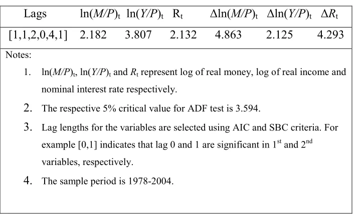
statistics for the levels and first differences of the variables are given in table 1 below :

Table 1: ADF Unit Root Tests

Lags ln(M/P)t ln(Y/P)t Rt ∆ln(M/P)t ∆ln(Y/P)t ∆Rt

[1,1,2,0,4,1] 2.182 3.807 2.132 4.863 2.125 4.293

Notes:

1. ln(M/P)t, ln(Y/P)t and Rt represent log of real money, log of real income and

nominal interest rate respectively.

2. The respective 5% critical value for ADF test is 3.594.

3. Lag lengths for the variables are selected using AIC and SBC criteria. For example [0,1] indicates that lag 0 and 1 are significant in 1st and 2nd variables, respectively.

4. The sample period is 1978-2004.

The null hypothesis of unit root cannot be rejected at the 5% level for the level variables

ie. ln(M/P)t, ln(Y/P)t, and Rt. Alternatively, the null that their first differences have unit

roots is clearly rejected. Therefore, the level variables are I(1) and their first differences are stationary. Microfit 4.1 is used for all estimations.

& $ # ! ' $ ' (

)$ *$ ## !)

In this section, we discuss our results obtained with the GETS approach where demand

for real narrow money is estimated with a lag structure of 4 periods. Using standard

variable deletion tests, these were later reduced to manageable parsimonious versions as

reported in Table-2. ∆2 lnPt captures the effects of the growth in expected inflation and it

has a negative coefficient. In Table-2, the equation GETS(1) is the initial parsimonious

version and GETS(2) is the constraint. The two crucial implied long-run elasticities for

income and the rate of interest are significant with correct signs and expected

could not reject the null that it is unity at the 5% level. The Wald test computed X2(1) test

statistic with p-value in parenthesis is 1.957 (0.162) is insignificant. Further, the

coefficients ∆Rt and ∆Rt-2 are close and opposite in sign. Likewise, the coefficients of

∆ln(M/P)t-3 and ∆ln(Y/P)t-2 are close but with same sign. When we tested for the

constraint with the Wald test, these constraints were accepted at the 5% level5. The equation GETS(2) are with these constraints.

Our preferred GETS equation for Tonga is GETS(2). The implied constraint income

elasticity for Tonga is unity and interest rate elasticity at mean interest rate of 5.92 is

-0.12. The adjusted R2is about 0.79 and a regression between the actual and fitted values of the change in logarithm of real money gives an intercept of zero and a slope of 1. The

SER is reasonable and the X2 summary statistics indicate that there is no serial correlation

X2sc,functional form misspecification X2ff, non-normality X2n and heteroscedasticity X2hs

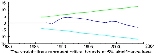
in the residuals. Our preferred equation GETS(2) is tested for temporal stability and

neither the CUSUM nor CUSUMSQUARES test showed any instability. This implies that the demand for money function is stable in Tonga. The plot of the stability test CUSUM

SQUARES is given in figure 1 below6.

Figure 1: Stability Test for Demand for Money (GETS)

! ! " " #

5

The Wald test computed X2(1) test statistics and p-values in parenthesis are 1.211(0.271) and 0.807(0.369)

respectively.

6

)$ + ' ## !)

The stationarity tests of ln(M/P)t, ln(Y/P)t and Rt using the ADF test indicated that they

are unit root in levels but are stationary in their first differences. The optimum lag lengths

of the VARs were tested with a 4th order model. The Akaike Information Criteria (AIC) and Schwartz Bayesian Criteria (SBC) criteria were used to select the lag length of the

VAR and both indicated lag length of 1 period. The test for determining the number of

cointegrating vectors is conducted with the Johansen maximum likelihood procedure in

Microfit 4.1. First, no intercept or trend option is used where the maximal eigenvalue and

trace test statistics for the null that there is no cointegration are 19.255 and 27.535

respectively. The 95% critical values, respectively, are 17.68 and 24.05. For the null that

there is one cointegrating vector, the corresponding computed values, with the critical

values in the parentheses are 7.531 (11.03) and 8.280 (12.36) respectively. Therefore, the

null hypothesis that there are no cointegration is rejected but the null that the number of

cointegrating vectors is one is not rejected. The implied cointegrating vector (CV)

normalized on ln(M/P)t is given below.

ln (M/P)t = 1.047 ln (Y/P)t - 0.038 Rt

(11.53)* (2.57)* (2)

The estimated income elasticity is around unity and the implied interest rate elasticity is

also significant and plausible. These are consistent with our GETS estimates given in

Table-2.

We proceed further for identification tests. Here the first difference of each variable is

regressed on their respective one period lagged residuals. When the CV is normalized on

real money, its residuals are denoted as ECMMt. Similarly, ECMYt and ECMRt are the

residuals of CVs normalized on income and the rate of interest, respectively. The

cointegrating vector represents long run demand for money function since only the

and ECMRt were insignificant in their respective regressions. The computed coefficients

for each of these lagged ECMs and their t-ratios in parenthesis are reported in the diagonals of the 3 x 3 matrices in Table-1A in the Appendix.

Further, endogeneity tests are conducted as pointed out by Enders (2004). Here three

different ECM equations are estimated to test the endogeneity. In each of the implied equation, ECMMt-1 term being included as one of the independent variable. We found

that the ECMMt-1 is only significant with the correct negative sign in the equation where

the dependent variable is ∆ln(M/P)t.The t-ratios for the ECMt-1 are along the first row in

the matrix, see Table-1A in the Appendix. Since the dis-equilibrium in the respective

money markets do not significantly contribute to the explanation of ln (Y/P)t and Rt, we

can treat ln (Y/P)t and Rt as being weakly exogenous variables7.

Now we estimate the dynamic money demand equation adopting the lag search procedure

used in the GETS equation in the second stage. We arrived at the parsimonious JML

equations reported in Table-2. The coefficient of the lagged error term have correct sign

and are significant at the conventional level. This implies the presence of negative

feedback mechanism. The growth in expected inflation is significant with correct sign.

The equations JML(1) is unconstraint and JML(2) is constraint version. We then tested if

the coefficients of ∆ln(Y/P)t-2, ∆ln(Y/P)t-4 and ∆2 lnPt-1 in JML(1) are close and the null is

accepted as the Wald computed X2(1) statistics (with p-value in parenthesis) of 2.155

(0.14) is insignificant. Similarly, we tested if there was any difference in the signs and

magnitudes of ∆Rt and ∆Rt-3. The constraint is also accepted as the X2(1) is 0.003 (0.96) is

insignificant. Therefore, JML(2) which is our preferred JML estimate for Tonga is

estimated with these restrictions and the results show an improvement over JML(1). The

X2 summary statistics of both JML equations are reasonable.

7

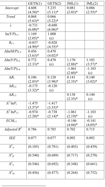
Table 2: Results obtained with GETS and JML8

GETS(1) GETS(2) JML(1) JML(2)

Intercept 4.608 (4.50)* 5.235 (5.11)* 0.081 (2.03)* 0.086 (2.55)*

Trend 0.068

(5.63)*

0.066 (5.22)*

λ -0.731

(6.08)*

-0.680 (6.06)* ln(Y/P)t-1 1.169

(2.05)*

1.000 (c) Rt-1 -0.037

(4.99)*

-0.020 (4.55)* ∆ln(M/P)t-3 0.456

(3.63)*

0.470 (4.02)* ∆ln(Y/P)t-2 0.772

(2.33)* 0.470 (c) 1.170 (2.88)* 1.103 (3.57)* ∆ln(Y/P)t-4 -1.061

(2.60)*

-1.103 (c) ∆Rt 0.106

(2.85)* 0.120 (3.98)* 0.141 (2.35)* 0.140 (3.02)* ∆Rt-2 -0.175

(3.32)*

-0.120 (c)

∆Rt-3 0.138

(2.35)*

0.140 (c) ∆2 lnPt -1.475

(3.57)*

-1.417 (3.53)* ∆2 lnPt-1 -0.974

(2.20)* -0.738 (2.14)* -1.061 (2.19)* -1.103 (c)

ECMt-1 -0.146

(4.04)*

-0.141 (4.05)*

Adjusted R2 0.786 0.785 0.702 0.715

SEE 0.077 0.077 0.092 0.092

X2sc (0.105) (0.781) (0.403) (0.439)

X2ff (0.540) (0.689) (0.717) (0.270)

X2n (0.546) (0.692) (0.348) (0.661)

X2hs (0.456) (0.477) (0.264) (0.752)

8

The plots of actual and predicted values of the change in the logarithm of real money

indicate fairly good fit. A regression between the actual and fitted values showed that the

intercept is zero and the slope is unity. The preferred equation JML(2) was tested for

temporal stability and neither the CUSUM nor CUSUM SQUARES test showed any instability. Here we obtained similar result as GETS that demand for money is stable in

Tonga. The plot of the stability test CUSUM SQUARES is given in figure 2 below9.

Figure 2: Stability Test for Demand for Money (JML)

$ $ $ $ $

! ! " " #

9

, ! !'

In this paper, we have estimated demand for real narrow money for Tonga. Both our

GETS and JML estimates gave similar and consistent results. We found that the demand

for money function in Tonga is temporally stable and well- determined. One of the

implication of our findings is that money supply is the appropriate monetary policy

instrument to be used by the National Reserve Bank of Tonga. The estimated income and

interest rate elasticities are well- determined and their signs and magnitudes are

consistent with prior expectations. Our results show that income elasticity is unity and the interest rate elasticity is negative and significant.

Finally, a few limitations of our work should be noted. First, there are limitations in the

data as a result we are unable to take long sample period. Second, we have ignored

structural breaks and their implications on unit root tests as implied by Perron (1989), as

these are outside the scope of this paper. Our purpose of this paper was only to

investigate stability of demand for money in Tonga. We hope our work is useful for

-- .

P = GDP deflator (1995=100). Data are derived from International Financial Statistics (IFS-2005).

Y = Nominal GDP at factor cost. Data are from (IFS-2005) and ADB database(2005).

R = The average of 1-3 years savings deposit rate. Data obtained from the (IFS-2005) and ADB database.

M1 = Currency in circulation and demand deposit. Data obtained from the (IFS-2005).

Notes:

1) All variables, except the rate of interest, are deflated with the GDP deflator and

converted to natural logs.

2) Data are available for replication on request.

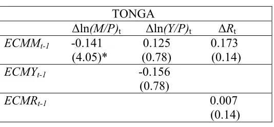
Table 1A: Identification and Exogeneity Tests

TONGA

∆ln(M/P)t ∆ln(Y/P)t ∆Rt

ECMMt-1 -0.141 0.125 0.173

(4.05)* (0.78) (0.14)

ECMYt-1 -0.156

(0.78)

ECMRt-1 0.007

(0.14)

Notes:

1. The t- ratios are reported below the coefficients. Significance at 5% is indicated by *.

2. ECMMt-1, ECMYt-1 and ECMRt-1 are the lagged residuals of the CVs normalized

Deadman, D. and Ghatak, S. (1981) “On the Stability of the Demand for Money in

India," Indian Economic Journal, 29(1), 41-54.

Enders, w., (2004) Applied Econometric Time Series, 2nd edition, (Hoboken NJ: John Wiely).

International Financial Statistics, December, 2005. IMF CD-ROM (Washington DC:

International Monetary Fund).

Jayaraman, T.K. and Ward, B.D., (2003) ``Impact of Financial Sector Reforms and

Stability of Money Demand Functions in Samoa," in Jayaraman, T.K., Issues in

Monetary Economics of the South Pacific Island Countries, Suva: The University of the

South Pacific.

Katafono, R. (2001)``Demand for Money in Fiji," Staff Working paper (03/2001). Suva: The Reserve Bank of Fiji.

Perron, P. (1989) “The Great Crash, the Oil Price Shock and the Unit Root Hypothesis,"

Econometrica, 57(6): 1361-1401.

Pesaran, M., and Pesaran, B. (1997) Working with Microfit 4.0. Oxford: Oxford University Press.

Poole, W. (1970) “The optimal choice of monetary policy instruments in a simple macro

model," Quarterly Journal of Economics, pp.192-216.

Rao, B.B and Kumar, S. (2006a) “Structural Breaks and the Demand For Money for Fiji,"

Rao, B.B and Singh (2005a) “Cointergration and Error Correction Approach to the

Demand for Money in Fiji," Pacific Economic Bulletin, (June): 72-86.

--- (2005b) “Demand for Money in Fiji with PcGets", Applied Economics

Letters, forthcoming.

Singh, R. and Kumar, S. (2006a) `` Cointegration and Demand For Money in Pacific

Island countries ," Staff Working Paper (3/2006). Suva: The University of the South Pacific.

Singh, R. and Kumar, S. (2006b) `` Demand For Money in Developing countries:

Alternative Estimates and Policy Implications," Staff Working Paper (5/2006). Suva: The University of the South Pacific.

Sriram, S. S., (1999) “Survey of literature on demand for money: Theoretical and

empirical work with special reference to error-correction models," IMF Working Paper

7WP/99/64 (Washington DC: International Monetary Fund).

The Asian Development Bank, (2005) ``Economic and Financial Update - 2005," Key

Indicators of Developing Asia and Pacific Countries. Manilla: The Asian Development