Spectral Boundary Integral Method
Thesis by
Ajay Bangalore Harish
In Partial Fulfillment of the Requirements
for the Degree of
Aeronautical Engineer
California Institute of Technology
Pasadena, California
2009
Acknowledgements
I consider myself exceptionally fortunate to have had the opportunity to work as a
Masters student at Caltech, working with a number of great scientists and wonderful
people. The time has finally come to say thanks to them.
Firstly I express my sincere gratitude to my advisor Prof. Nadia Lapusta for all the
guidance, inspiration and support. Nadia introduced me to the field of dynamic
frac-ture mechanics and had remarkable patience to spend hours going through research
and was always willing to help me see connections between seemingly unrelated
re-sults and make everything fit together. This thesis would not have been possible
without her critical contributions and insights.
I would also like to thank Prof. Guruswami Ravichandran and Prof. Chiara Daraio
for graciously agreeing to be on my thesis committee, reviewing my thesis and
pro-viding crucial criticisms and suggestions. Prof. Ravichandran has given me constant
support throughout my stay at Caltech. I would also like to thank Prof. Ares Rosakis
for the critical insights into the problem.
I would also like to extend my sincere appreciation to my group members - Dr. Yi
Liu, Dr. Xiao Lu, Dr. Yoshihiro Kaneko, Ahmed Elbanna and Ting Chen for all the
help and support in the last year of stay at Caltech. I specially thank Dr. Yi Liu
for providing his 3D code for dynamic shear ruptures on bimaterial interfaces that
served as a starting point for the code developed in my work. I am also grateful to
data for comparison with my modeling. I also thank Maria for all the help extended.
I also like to thank Dr. Harsha Bhat and Mike Mello for all the help and constant
advice and suggestions throughout my stay at Caltech. I would also like to extend my
appreciation to all my office mates - Bharat Prasad, Phanish Suryanarayana, Daniel
Hurtado for all the help. I would also like to thank my colleagues for all the
study-ing we did in the SFL library - Prakhar Mehrotra, Sandeep Kumar Lahiri, Nicholas
Boecler, Michio Inoue, Kawai Kwok, Inki Choi, Devvrath Khatri, Celia Reina Roma,
Vahe Gabuchian, Jon Mihaly. I also thank my co-TA’s Farshid Roumi and Timothy
Kwa was making the teaching experience of ME-35 a memorable one. I also thank all
my other friends at Caltech who made my stay academically and socially stimulating
and to name some - Sujit Nair, Rajani Kurup, Navneet T Narayan, Manav Malhotra,
Deb Ray. I whole-heartedly thank everyone who has been of help knowingly and
unknowingly.
Last but never the least I whole-heartedly thank my parents for standing by me,
believing in me and supporting all my decisions unconditionally through the hard
Abstract
Simulation of three-dimensional dynamic fracture events constitutes one of the most
challenging topics in the field of computational mechanics. Spontaneous dynamic
fracture along the interface of two elastic solids is of great importance and interest
to a number of disciplines in engineering and science. Applications include dynamic
fractures in aircraft structures, earthquakes, thermal shocks in nuclear containment
vessels and delamination in layered composite materials.
This thesis presents numerical modeling of laboratory experiments on dynamic shear
rupture, giving an insight into the experimental nucleation conditions. We describe a
methodology of dynamic rupture simulation using spectral boundary integral method,
including the theoretical background, numerical implementation and cohesive zone
models relevant to the dynamic fracture problem. The developed numerical
imple-mentation is validated using the simulation of Lamb’s problem of step loading on an
elastic half space and mode I crack propagation along a bonded interface. Then the
numerical model and its comparison with experimental measurements is used to
in-vestigate the initiation procedure of the dynamic rupture experiments. The inferred
parameters of the initiation procedure can be used in future studies to model the
Contents
Acknowledgements i
Abstract iii
Contents v
List of Figures x
List of Tables x
1 Introduction 1
1.1 Goal and outline . . . 1
1.2 Description of experiments that motivate our modeling . . . 3
1.2.1 Configuration of the experiment . . . 4
1.2.2 Rupture nucleation mechanism . . . 5
1.3 Relevant experimental observations . . . 7
2 Spectral Boundary Integral Method And Its Numerical Implemen-tation 9 2.1 Introduction to dynamic fracture simulations . . . 9
2.2 Theoretical formulation of the spectral boundary integral method . . 11
2.3 Numerical implementation of the spectral scheme . . . 18
2.4 Theoretical formulation of cohesive zone laws . . . 22
2.4.1 Ortiz-Camacho Model . . . 23
3 Validation of the developed numerical approach 26
3.1 Study of Lamb’s problem on an elastic half-space . . . 26
3.1.1 Theoretical formulation of Lamb’s problem . . . 26
3.1.2 Numerical investigation of Lamb’s problem . . . 28
3.2 Propagating mode-I crack in a plate . . . 31
3.2.1 Critical crack length . . . 31
3.2.2 Cohesive zone length . . . 34
3.2.3 Numerical resolution . . . 35
3.2.4 Numerical simulation of propagating mode I crack in rocks . . 36
4 Simulations of nucleation procedure in laboratory earthquake exper-iments 41 4.1 Comparison of numerically computed and experimentally measured interface-parallel displacements . . . 42
4.1.1 Effect of the explosion pressure . . . 43
4.1.2 Effect of the cohesive zone models . . . 49
4.1.3 Effect of loading duration . . . 51
4.1.4 Effect of plasma spreading speed (Cpla) . . . 54
4.2 Mode I crack propagation due to the nucleation procedure . . . 56
4.3 Conclusions . . . 58
4.4 Future work . . . 64
List of Figures
1.1 Experimental Setup. Adapted from Lu (2009) . . . 4
1.2 Schematic diagram of the exploding wire system coupled with a
photoe-lastic fault model. Adapted from Xia (2005) . . . 6
1.3 Comparison of the experimentally measured interface-parallel
displace-ment for 0-degree and 90-degree points. Adapted from Lu (2009) . . . 8
1.4 Comparison of the experimentally measured interface-parallel velocity
for 0-degree and 90-degree points. Adapted from Lu (2009) . . . 8
2.1 Problem Geometry . . . 11
2.2 Convolution kernels in displacement formulation for a Poisson ratioν=
0.35 . . . 18
2.3 Convolution kernels in velocity formulation for a Poisson ratio ν= 0.35 19
2.4 Tensile cohesive relation - Ortiz-Camacho cohesive relation . . . 24
2.5 Reversible rate-independent cohesive model . . . 25
3.1 Evolution of displacement normal to the traction-free surface at a point
located at a distance L from the point of application of load. Dotted
lines denote the arrival times of dilatational, shear and Rayleigh waves. 29
3.2 Displacement field on the surface of the half space after 200 time steps,
showing the concentric waves expanding from the point of application
of point load . . . 30
3.3 A funnel crack in a plate subjected to external loads. . . 32
3.4 Propagation of mode I crack across the domain with time (0, 0.10, 0.20,
3.5 Propagation of mode I crack across the domain with time (0.35, 0.40,
0.45, 0.50 μs) . . . 38
3.6 Propagation of mode I crack across the domain with time (1, 2, 3, 4 μs) 39
3.7 Propagation of mode I crack across the domain with time (5, 6, 7, 8 μs) 39
4.1 The pressure profile used to model the explosion. Pmax is the maximum
pressure. t1, t2 and t3 are the time parameters of the loading profile. . 44
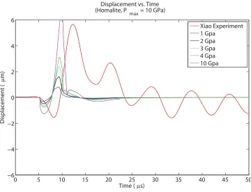
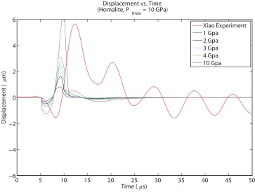
4.2 Comparison of interface-parallel displacement at a distance of 10 mm
from the point of explosion for loading profile 2 and parameters Pmax = 1,2,3,4,10 GPa and t1 = 0μ, t2 = t3 = 5μs. The numerical simulation
being governed by Ortiz-Camacho cohesive zone model. . . 45
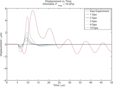
4.3 Comparison of interface-parallel displacement at a distance of 10 mm
from the point of explosion for loading profile 2 and parameters Pmax = 1,2,3,4,10 GPa and t1 = 0μ, t2 = t3 = 5μs. The numerical simulation
being governed by reversible rate-independent cohesive zone model. . . 46
4.4 Comparison of interface-parallel displacement at a distance of 10 mm
from the point of explosion for loading profile 2 and parameters Pmax = 1,2,3,4,10 GPa and t1 = 0μ, t2 = 4μs, t3 = 5μs. The numerical
simulation being governed by Ortiz-Camacho cohesive zone model. . . 47
4.5 Comparison of interface-parallel displacement at a distance of 10 mm
from the point of explosion for loading profile 2 and parameters Pmax
= 1,2,3,4,10 GPa and t1 = 0μ, t2 = 4μs, t3 = 5μs. The numerical simulation being governed by reversible rate-independent cohesive zone
model. . . 48
4.6 Comparison of interface-parallel displacement, for numerical simulations
governed by Ortiz-Camacho cohesive zone model and reversible
rate-independent cohesive zone model, at a distance of 10 mm from the point
of explosion for loading profile 1 with parameters Pmax = 10 GPa and
4.7 Comparison of interface-parallel displacement, for numerical simulations
governed by Ortiz-Camacho cohesive zone model and reversible
rate-independent cohesive zone model, at a distance of 10 mm from the point
of explosion for loading profile 2 with parameters Pmax = 10 GPa and
t1 = 0μ, t2 = 4μs, t3 = 5μs. . . 50
4.8 Comparison of interface-parallel displacement, for numerical simulations
governed by Ortiz-Camacho cohesive zone model, at a distance of 10 mm
from the point of explosion for loading profile 1 with parameters Pmax = 10 GPa and t1 = 1,2,3,4 μ, t2 - t1 = 3 μs and t3 - t2 = 1 μs. . . 52
4.9 Comparison of interface-parallel displacement, for numerical simulations
governed by Ortiz-Camacho cohesive zone model, at a distance of 10 mm
from the point of explosion for loading profile 1 with parameters Pmax = 10 GPa and t1 = 2 μ, t2 - t1 = 3,4,5 μs and t3 - t2 = 1 μs. . . 53
4.10 The best match between the simulations and the experimental results.
The parameters used are Pmax = 10 GPa, t1 = 2 μs, t2 - t1 = 4 μs, t3
-t2 = 1 μs and Cpla = crack tip speed. . . 54
4.11 Comparison of interface-parallel displacement, for numerical simulations
governed by Ortiz-Camacho cohesive zone model, at a distance of 10 mm
from the point of explosion for loading profile plasma speeds of Cpla =
250 m/s, 340 m/s, 500 m/s. The loading parameters are Pmax = 10
GPa, t1 = 1 μ, t2 = 4 μs,t3 = 5 μs . . . 55 4.12 Opening velocity in the nucleation region (at t= 0,25,50,75 ns) . . . . 56
4.13 Opening velocity in the nucleation region (at t= 0.1,0.2,0.3,0.4μs) . . 57
4.14 Opening velocity in the nucleation region (at t= 0.5,0.6,0.7,0.8μs) . . 57
4.15 Opening displacement in the nucleation region (at t= 0,25,50,75 ns) . 58
4.16 Opening displacement in the nucleation region (att = 0.1,0.2,0.3,0.4μs) 59
4.17 Opening displacement in the nucleation region (att = 0.5,0.6,0.7,0.8μs) 60
4.18 Opening velocity in the domain (at t= 1,2,3,4 μs) . . . 61
4.19 Opening velocity in the domain (at t = 5,6,7,8 μs) . . . 61
4.21 Opening displacement in the domain (at t = 1,2,3,4 μs) . . . 62
4.22 Opening displacement in the domain (at t = 5,6,7,8 μs) . . . 63
List of Tables
1.1 Summary of mechanical properties of Homalite-100 . . . 5
3.1 Numerical resolution of critical crack length and cohesive zone length
for various levels of prestress . . . 36
Chapter 1
Introduction
1.1
Goal and outline
Modeling and simulation of dynamic fracture events is an important topic of
com-putational and experimental mechanics. Dynamic fracture is especially important in
the field of geophysics, in the simulation of earthquakes. Earthquakes are destructive
processes that occur as dynamical ruptures along the pre-existing faults (interfaces)
in the Earth’s crust. The practical goal of earthquake seismology is to prevent or
re-duce human and material losses by estimating the earthquake hazard at a given site
or by forecasting the occurrence of the next strong event. Detailed seismic inversions
have significantly improved our understanding of earthquake rupture processes. But
yet the progress has been less due to the fact that Earth is a complex system.
This highlights the necessity for controlled laboratory experiments and extensive
nu-merical modeling of the dynamic rupture process along an interface. One example of
such experiments is work of Xia et al. (2004) which demonstrated, for the first time, the transition of shear mode II ruptures from sub-Rayleigh to supershear speeds.
Further experiments were conducted by Lu et al. (2009), Lu (2009) to study the su-pershear transition and rupture modes. An approximate numerical modeling of the
experiment was developed by Luet al. (2009).
giving an insight into the experimental nucleation conditions. In chapter 1, we present
a review of the experimental techniques used in the laboratory dynamic rupture
exper-iments and relevant experimental observations. In chapter 2, we discuss the
method-ology of dynamic rupture simulation using spectral-boundary integral method - both
theoretical formulation and numerical implementation. Also in the same chapter we
discuss the various cohesive laws relevant to the dynamic fracture problem. In chapter
3, the numerical model developed in chapter 2 is validated using a half-space
simula-tion of Lamb’s problem. In chapter 4, the numerical model is used for investigating
the initiation procedure in dynamic rupture experiments (Xia (2005), Lu (2009)).
Using conceptual loading profiles, we determine the propagation of an opening mode
due to the explosive initiation procedure and compare our simulations with
experi-mental results of Lu (2009). In chapter 5, we discuss the conclusions of the work and
directions for future work.
Understanding whether supershear transition observed in rupture experiments (Xia
et al.(2004), Luet al.(2009)) is affected by nucleation procedure is the ultimate goal of the present work. Supershear transition has been a topic of research dating back
to early 70’s (Burridge (1973); Andrews (1976); Das & Aki (1977); Burridge et al.
(1979); Freund (1979); Day (1982); Broberg (1989); Needleman & Rosakis (1999);
Abraham & Gao (2000); Madariaga & Olsen (2000); Gao et al. (2001); Geubelle & Kubair (2001); Dunham & Archuleta (2005); Festa & Vilotte (2006); Rosakis et al.
(2007); Liu & Lapusta (2008); Shi et al. (2008)). The occurrence of supershear tran-sition has been inferred from observations of large earthquakes. This has been further
confirmed in the laboratory (Xiaet al. (2004), Lu (2009)) and numerical models have been developed to approximately simulate the experiments (Lu et al.(2009)).
We numerically model the effects of experimental nucleation procedure using spectral
boundary-integral method (BIM). Boundary integral methods have been widely used
to investigate spontaneous propagation of cracks in elastic media (e.g., Das (1980);
(2000)). Formulations discussed by Perrin et al. (1995) and Geubelle & Rice (1995) allowed for 3D dynamic crack propagation in a homogeneous linearly elastic solid.
Further formulations of Geubelle & Breitenfeld (1997) and Breitenfeld & Geubelle
(1998) extended the earlier formulations and dealt with the problem of dynamic
crack propagation on bimaterial interfaces accounting for both tangential and normal
displacements of the fracture surface.
One of the approaches to modeling fracture is based on cohesive zone models. The
idea of a crack tip cohesive zone was first proposed by Barenblatt (1959). A similar
model was suggested by Dugdale (1960) to account for the plastic zone at the crack
tip. The physical motivation for postulating a cohesive model is different in different
applications but the form of cohesive models is similar in all cases. The fracture is
regarded as a gradual process in which the separation is resisted by cohesive
trac-tions. The relationship between the cohesive traction and the opening displacement
is governed by a cohesive law. The cohesive zone models used in problems of dynamic
crack growth include the cohesive models developed by Camacho & Ortiz (1996) and
Xu & Needleman (1994).
The algorithm developed has been tested in the case of the Lamb’s problem of step
loading on a half space by a concentrated normal force on its boundary. The original
formulation of the problem was by Lamb (1904). The numerical solutions were also
directly compared with the closed form analytical solutions to the Lamb’s problem
was given by Pekeris (1955).
1.2
Description of experiments that motivate our
modeling
In this section, we describe the experimental setup and techniques developed by Xia
governing the rupture dynamics of crustal earthquakes while still preserving enough
simplicity to make conclusions by direct observation.
1.2.1
Configuration of the experiment
The experimental setup mimics a fault in the Earth’s crust. The crust is simulated by
a large Homalite plate of dimensions 150mm×150mm×10mm (Figure 1.1). Relevant
properties of Homalite-100 are listed in the Table. 1.1 from Lu (2009). The Homalite
plate is cut into two identical quadrilaterals and are put together to introduce a
frictional interface. The interface has an inclination angleαwith respect to one of the
plate edges. The frictional interface is used to simulate a fault. A uniaxial pressure
(P) acts uniformly on the top and the bottom ends of the sample. Experimental
parameters (P and α) determine the resolved shear traction τ = Psinαcosα and
resolved normal traction σ =P cos2α along the fault. Varying α allows to vary the nondimensional fault prestressτ /σ = tanα and study its effects on rupture dynamics
and varying P allows for the study of the effect of absolute prestress.
Reflective Membranes
Polarized Laser Beam
Collimator
Laser
Circular Polarizer I
Leads
Capacitor Bank Exploding
Wire Circular Polarizer II
Laser Beams
Laser Heads
Pressure P
P Velocimeter Controller
Focusing Lens
High Speed Camera
[image:15.612.111.534.367.583.2]C1 C2
Material Property Homalite-100
Young’s modulus E (MPa) 3860
Shear modulus μ(MPa) 1429.63
Shear wave speed cs (m/s) 1078.10
Dilatational wave speed cp (m/s) (Plane-strain) 2244.24
Dilatational wave speed cp (m/s) (Plane-stress) 1891.11
Poisson ratio 0.35
Density ρ (kg/m3) 1230
Table 1.1: Summary of mechanical properties of Homalite-100
1.2.2
Rupture nucleation mechanism
The triggering of a natural earthquake can be achieved either by increase of the shear
loading or by decrease of the fault strength at a specific location. Both mechanisms
have been applied in numerical simulations of earthquake rupture dynamics (Andrews
(1976); Andrews & Ben-Zion (1997); Cochard & Rice (2000); Aagaardet al. (2001)).
In the experiments, the dynamic rupture is initiated by means of explosion of a thin
nickel wire as shown in Figure 1.2. A nickel wire with a diameter of 0.08 mm is
em-bedded within a 0.1 mm hole through the thickness of the entire plate. The ends of
the wire are connected to a capacitor (15μF) that is charged by a high voltage power
supply (1-3 kV). Upon closing the switch, the electric energy stored in the capacitor
causes a high current in the thin nickel wire for a short duration. The high current
turns the nickel wire into high temperature, high pressure plasma. The explosion
either changes fault normal pressure to tensile and drives the dynamic rupture as a
mixed-mode rupture or reduces it locally and facilitates a pure mode II rupture along
the interface.
Figure 1.2: Schematic diagram of the exploding wire system coupled with a photoe-lastic fault model. Adapted from Xia (2005)
by Xia (2005) using the Gr¨uneisen equation of state:
p0−px= γ (v)
v (E−Ex) (1.1)
where γ is the Gr¨uneisen parameter (approximately 1.88 for Nickel), E and Ex are
the total internal energy and cold internal energy, p0 and px are the total pressure and cold pressure andv is the volume of the material. The cold pressure and the cold
energy are due to the mechanical interaction of atoms and are negligible. The total
energy supplied by the capacitor is
Etotal = CV
2
2 (1.2)
For a case of V = 1 kV, the total energy is 7.5 J. Assuming losses of the order of 1 J
due to wire expansion, from (1.1) we can calculate the peak pressure of the order of
10 GPa. In the subsequent chapters we study the effect of the nucleation procedure
1.3
Relevant experimental observations
Detailed experiments were conducted by Lu (2009) to understand the nucleation
con-ditions due to the explosion procedure. The diagnostic methods used were dynamic
photoelasticity and laser velocimetry. In addition to photoelastic imaging, two laser
velocimeters were used to measure the particle velocity histories of two points, one
above and one below the fault interface. Experiments were conducted on interfaces
of zero inclination and the particle velocities were measured at a distance of 10 mm
from the point of explosion. Particle velocities measured included fault-parallel
ve-locity along the interface and fault-normal veve-locity at a point directly above the point
of explosion.
One set of such measurements (Lu (2009)) is shown in Figures 1.3 & 1.4. If the
explo-sion were axisymmetric, the response of both points would be the same but different
response was observed during the experiments (Figures 1.3 & 1.4). Thus one could
infer the possibility of a mode I crack opening due to explosion.
The aim of this thesis is to extend the existing code for modeling shear ruptures
(Lapusta et al. (2000), Day et al. (2005), Lu et al. (2009)) to include the mode I component and to use the developed code and experimental measurements of Lu
(2009) to infer parameters of the initiation procedure. These parameters can be used
in future studies to model the experimental results on supershear transition (Xia
0 20 40 60 80 100 −13
−11 −9 −7 −5 −3 −1 1 3 5 7 9 11 13
Time (μs)
Interface−parallel displacement
(
μ
m)
Interface−parallel displacement
[image:19.612.151.484.41.280.2](At a distance of 10 mm from point of explosion. Prestress = 8.7MPa) 90 degree displacement ( μm) 0 degree displacement ( μm)
Figure 1.3: Comparison of the experimentally measured interface-parallel displace-ment for 0-degree and 90-degree points. Adapted from Lu (2009)
0 20 40 60 80 100
−4 −3 −2 −1 0 1 2 3 4
Time (μs)
Interface−parallel velocity (m/s)
Interface−parallel velocity
(At a distance of 10 mm from point of explosion. Prestress = 8.7MPa) 90 degree velocity (m/s) 0 degree velocity (m/s)
[image:19.612.160.487.360.612.2]Chapter 2
Spectral Boundary Integral
Method And Its Numerical
Implementation
2.1
Introduction to dynamic fracture simulations
Dynamic fracture mechanics simulations and the problem of spontaneously
propagat-ing cracks have been an important area of fracture mechanics research in engineerpropagat-ing
and geophysics. Dynamic fracture mechanics simulations require high degree of
refine-ment in spatial and temporal discretization to accurately represent the rapid changes
in field variables associated with traveling crack tips and elastic waves. On the other
hand, large domains of analysis are required to reduce the interactions due to domain
boundaries. This results in a substantial challenge in terms of computational cost.
Various numerical techniques have been developed over the years to investigate the
problem of spontaneous crack propagation, including finite element and finite
dif-ference methods (e.g., Ortiz & Pandolfi (1999), Yu et al. (2002), Templeton et al.). However both methods incorporate simulation of wave propagation in the bulk, which
makes them applicable to problems with heterogeneous bulk but computationally
ex-pensive. For dynamic rupture of plane interfaces embedded in a uniform elastic space,
boundary integral methods have emerged as the most accurate and efficient choice
(1994), Geubelle & Rice (1995), Perrinet al.(1995), Ben-Zion & Rice (1997), Geubelle & Breitenfeld (1997), Kame & Yamashita (1999), Aochiet al. (2000), Lapusta et al.
(2000), Lapusta & Rice (2000), Dayet al. (2005)). The boundary integral method is based on restricting the consideration to the interface plane. The elastodynamic
re-sponse of the surrounding elastic media is expressed in terms of integral relationships
between interface displacements and tractions. These integral relationships involve
convolutions of space and time of displacement discontinuities and histories. The
histories are obtained through integral relationships between displacement
disconti-nuities and convolution kernels. The convolutions account for the wave propagation
and are analytically derived through closed-form Green function. This eliminates the
need to simulate the wave propagation through elastic media.
In the study of anti-plane shear study of a slip on a planar fault, Perrin et al.(1995) adopted the spectral representation of a slip distribution as a Fourier series in the
space coordinate along the fracture plane, instead of dealing with the approximations
to the space-time convolution integral, as in standard BIM. In this work, we follow
Perrin et al. (1995) in adopting the spectral representation of the relation between the tractions and the resulting discontinuities.
The spectral scheme has been developed over the years (Perrinet al.(1995); Geubelle & Rice (1995); Geubelle & Breitenfeld (1997); Breitenfeld & Geubelle (1998), Day
et al.(2005)). It provides an attractive alternative for the simulation of spontaneous crack propagation. The spectral formulation allows one to study in great detail the
spontaneous initiation, propagation, and arrest of one or more planar cracks and
faults embedded in an infinite medium and subjected to space- and time-varying
dy-namic loading. It provides a major advantage in comparison with the conventional
boundary integral method. The spectral scheme involves a convolution in time as the
dynamic stresses are computed in the spectral domain while the conventional scheme
2.2
Theoretical formulation of the spectral
bound-ary integral method
The spectral formulation is based on the Fourier representation of stresses and
dis-placements in spatial coordinates along a fracture plane in an infinite, homogeneous,
linearly elastic body. The formulation embodies an exact elastodynamic
representa-tion of the relarepresenta-tion existing between the Fourier coefficients of tracrepresenta-tions and
corre-sponding displacement discontinuities. In this section, we give the theoretical
formu-lation of the spectral method for the two-dimensional case following Breitenfeld &
Geubelle (1998).
X
3X
X
12
crack
[image:22.612.207.427.268.495.2]unbroken
Figure 2.1: Problem Geometry
Let the Cartesian coordinates be defined as shown in Figure 2.1 such that the
frac-ture plane coincides with x2 = 0. Hence x1 and x3 are coordinates in the plane and elastodynamic fields will exist in the adjoining half spaces x2 >0 and x2 <0.
Considering a 2D formulation, we consider that the displacements and the stress fields
stress and displacement field, respectively. LetTα(t :q) and Uα(t :q) denote theq
th-mode Fourier coefficients of the in-plane traction stresses and displacements such
that:
σ2α(x1,0±, t) = Tα(t;q)eiqx1
u±α(x1,0±, t) = Uα±(t;q)eiqx1
(2.1)
The first two components of the displacement field ui(xα, t) can be expressed as:
u1(xα, t) = φ,1(xα, t) +ψ,2(xα, t)
u2(xα, t) = φ,2(xα, t)−ψ,1(xα, t)
(2.2)
where the potentials φ and ψ satisfy the wave equations:
c2dφ,αα=φ,tt
c2sψ,αα =ψ,tt
(2.3)
while the third displacement component is such that
c2su3,αα=u3,tt (2.4)
Considering one particular spectral component
[φ(xα, t), ψ(xα, t), u3(xα, t)] =eiqx1[Φ(x
2, t;q),Ψ(x2, t;q),Ω(x2, t;q)] (2.5)
Now introducing the Laplace transform, the scalar wave equations (2.3) and (2.4)
reduce to:
ˆ
Φ(x2, p;q) = q2αd2Φ(x2, p;q) ˆ
Ψ(x2, p;q) = q2αs2Ψ(x2, p;q) ˆ
Ω(x2, p;q) = q2αs2Ω(x2, p;q)
where
( ) =∂/∂x2
αd =
1 + p
2
q2c2d, αs =
1 + p
2
q2c2s
(2.7)
Bounded solutions for (2.6) for x2 > 0 has the form as in (2.8). Similar analogous solution can be derived for x2 <0.
ˆ
Φ(x2, p;q) = ˆΦ0(p;q)e−|q|αdx2 ˆ
Ψ(x2, p;q) = ˆΨ0(p;q)e−|q|αsx2
ˆ
Ω(x2, p;q) = ˆΩ0(p;q)e−|q|αsx2
(2.8)
Combining the equations (2.2), (2.5) and (2.8), the Laplace-transformed displacement
field for the particular mode is given to be:
ˆ
u1(xα, p) =eiqx1
iqΦˆ0(p;q)e−|q|αdx2 − |q|α
sΨˆ0(p;q)e−|q|αsx2
ˆ
u2(xα, p) =eiqx1
−|q|αdΦˆ0(p;q)e−|q|αdx2 −iqΨˆ0(p;q)e−|q|αsx2
ˆ
u3(xα, p) =eiqx1Ωˆ0(p;q)e−|q|αsx2
(2.9)
We are concerned with the tractions acting along the fracture plane x2 = 0 and
the resulting displacements. Considering the Fourier coefficients as defined in (2.1),
relations (2.9) reduce to:
ˆ
U1(p;q) =iqΦˆ0(p;q)− |q|αsΨˆ0(p;q) ˆ
U2(p;q) =−|q|αdΦˆ0(p;q)−iqΨˆ0(p;q)
which can be inverted to obtain
ˆ
Φ0(p;q) = −iq ˆ
U1(p;q) +|q|αsUˆ2(p;q)
q2(1−αsαd)
ˆ
Ψ0(p;q) = |q|αd ˆ
U1(p;q) +iqUˆ2(p;q)
q2(1−αsαd)
(2.11)
Using (2.10) and (2.11) in (2.9), we obtain the solution for the displacement fields
ˆ
ui(xα, p) for the upper half space in terms of the components ˆUi(p;q) along the upper
side x2 = 0+ of the fracture plane.
ˆ
u1(xα, p) =eiqx1
ˆ
U1(p;q)e
−|q|αdx2 −α
sαde−|q|αsx2
1−αsαd
+ ˆU2(p;q) iqαs |q|(1−αsαd)
e−|q|αdx2 −e−|q|αsx2
ˆ
u2(xα, p) =eiqx1
ˆ
U1(p;q)| iqαd
q|(1−αsαd)
e−|q|αdx2 −e−|q|αsx2
+ ˆU2(p;q)e
−|q|αsx2 −α
sαde−|q|αdx2
1−αsαd
(2.12)
Now using (2.1) and (2.12) the Fourier coefficients of the traction components of the
two half spaces can be obtained to be:
ˆ
T1(p;q) =∓μ±|q|α
±
d(1−α±
2
s )
1−αs±α±d ˆ
U1±(p;q) +iμ±q 2−
1−αs±2 1−α±sα±d
ˆ
U2±(p;q)
ˆ
T2(p;q) =−iμ±q 2− 1−α
±2
s 1−α±sα±d
ˆ
U1±(p;q)∓μ±|q|α
±
d(1−α±
2
s )
1−α±sα±d ˆ
U2±(p;q)
(2.13)
by:
[ ˆT1]inst=∓μ
±
c±s p
ˆ
U1±(p;q)
[ ˆT2]inst=∓c
±
d
c±s2μ
±pUˆ±
2 (p;q)
(2.14)
Now rewriting (2.13) we obtain the expressions for Fourier coefficients of traction
components
ˆ
T1(p;q) =−μ
±
c±s
pUˆ1±(p;q)∓μ±|q|
αd±(1−α±s2) 1−α±sα±d −
p |q|c±s
ˆ
U1±(p;q)
+iμ±q
2− 1−α
±2
s 1−α±sα±d
ˆ
U2±(p;q)
ˆ
T2(p;q) =∓c
±
d
c±s
μ±pUˆ2±(p;q)∓μ±|q|
α±s(1−α±s2) 1−α±sα±d −
c±d c±s
p |q|c±s
ˆ
U2±(p;q)
−iμ±q
2− 1−α
±2
s 1−α±sα±d
ˆ
U1±(p;q)
(2.15)
Thus in the space-time domain we have the 2D elastodynamic relations, between the
traction components of the stress (τα) acting on the fracture plane and the resulting
displacements (u±α), are given by:
τ1(x1, t) =τ10(x1, t)∓ μ
±
c±s
∂u1(x1, t)
∂t +f
±
1 (x1, t)
τ2(x1, t) =τ20(x1, t)∓ c
±
d
c±s μ± c±s
∂u2(x1, t)
∂t +f
±
2 (x1, t)
(2.16)
The Fourier coefficients of the functional are related to the displacement
discontinu-ities through the convolution kernels and are given by
F1(t;q) =±μ±|q|
t
0
H11(|q|c±st)U1±(t−t;q)|q|c±s dt
+i(2−η±)μ±qU2±(t;q)
+iμ±q t
0
H12(|q|c±st)U2±(t−t;q)|q|c±s dt
F2(t;q) =∓μ±|q|
t
0
H22(|q|c±st)U2±(t−t;q)|q|c±s dt
−i(2−η±)μ±qU1±(t;q)
−iμ±q
t
0
H12(|q|c±st)U1±(t−t;q)|q|c±s dt
(2.17)
where η=cd/cs.
This formulation is known as the “Displacement Formulation” because the
convo-lutions are done on the histories of the Fourier coefficients of displacement
discon-tinuities. To separate the static (long-term) and transient dynamic responses, the
integrals in (2.17) are integrated by parts to obtain the Velocity Formulation (Perrin
are given to be:
F1(t;q) =±μ±|q| ⎡ ⎣L11U±
1 −
t
0
K11(|q|c±st) ˙U1±(t−t;q)dt
⎤ ⎦
+iμ±q
⎡ ⎣L12U±
2 −
t
0
K12(|q|c±st)U2±(t−t;q)dt
⎤ ⎦
+i(2−η±)μ±qU2±(t;q)
F2(t;q) =±μ±|q| ⎡ ⎣L22U±
2 −
t
0
K22(|q|c±st) ˙U2±(t−t;q)dt
⎤ ⎦
+iμ±q
⎡ ⎣L12U±
1 −
t
0
K12(|q|c±st)U1±(t−t;q)dt
⎤ ⎦
−i(2−η±)μ±qU1±(t;q)
(2.18)
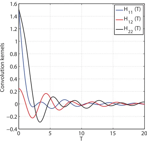
The Kernels in Displacement Formulation (H11, H12 and H22) are as calculated in Breitenfeld & Geubelle (1998) and the Kernels in Velocity Formulation, K11, K12,
K22, are given to be:
K11=L11−
T
0
H11(η)dη
K12=L12−
T
0
H12(η)dη
K22=L22−
T
0
H22(η)dη
where L11, L12 and L22 are given to be:
L11=
∞
0
H11(η)dη
L12=
∞
0
H12(η)dη
L22=
∞
0
H22(η)dη
(2.20)
0 5 10 15 20
−0.4 −0.2 0 0.2 0.4 0.6 0.8 1 1.2 1.4
Convolution kernels ( ν = 0.35)
T
Convolution kernels
H
11 (T)
H
12 (T)
H
[image:29.612.201.437.223.466.2]22 (T)
Figure 2.2: Convolution kernels in displacement formulation for a Poisson ratio ν = 0.35
The displacement convolution kernels and velocity convolution kernels are presented
in Figure 2.2 and Figure 2.3 respectively for a Poisson’s ratio ν = 0.35
2.3
Numerical implementation of the spectral scheme
The implementation of the 2D spectral formulation in this work is based on the
0 5 10 15 20 −0.4 −0.2 0 0.2 0.4 0.6 0.8 1 1.2 1.4 1.6
Convolution Kernels ( ν = 0.35)
T
Convolution kernels
H
11 (T)
H
12 (T)
H
[image:30.612.198.437.36.266.2]22 (T)
Figure 2.3: Convolution kernels in velocity formulation for a Poisson ratio ν = 0.35
(1998), Day et al. (2005) and Liu (2009). It starts by expressing the u±j and fj± distributions on the fracture plane as a double Fourier series with period X in thex1 direction such that
⎧ ⎨ ⎩
u±j(x1, t)
fj±(x1, t)
⎫ ⎬ ⎭=
K/2
q=−K/2
⎧ ⎨ ⎩
Ujk±(t)
Fjk±(t)
⎫ ⎬ ⎭e2πi(
kx1
X ) (2.21)
A conventional FFT algorithm is used to link spatial and spectral representations,
with K sampling points distributed uniformly over theX cells of the fracture plane.
Once the convolution term is computed using (2.18) in the spectral domain and
trans-fered back to the spatial domain, (2.16) is used to calculate the updated velocities
˙
u±k(x1, t). This is then integrated in time with an explicit scheme to derive the dis-placement field.
ua±j (x1, t+ Δt) =u±j(x1, t) + Δtu˙±j (x1, t) (2.22)
during the first iteration.
ub±j (x1, t+ Δt) =u±j (x1, t) + 0.5Δt
˙
u±j(x1, t) + ˙ua±j (x1, t+δt)
during the second iteration. uaj and ubj represent the displacements from first and
second iterations respectively. ˙uaj and ˙ubj represent the velocities from the first and
second iterations respectively.
The time step Δt is chosen to be a fraction of time needed for the shear wave to
propagate the smallest distance between the grid points defined on the fracture plane
as
Δt=β Δx
max(c+s, c−s) (2.24)
The user-defined parameterβ plays a critical role in stability and precision of the
nu-merical scheme for the bimaterial code as discussed in Breitenfeld & Geubelle (1998).
Continuity conditions are incorporated along the interface plane and a cohesive failure
model is introduced to allow for spontaneous propagation of an interface crack. The
failure models discussed in this work are the Camacho-Ortiz Model (Camacho &
Or-tiz (1996)) and a reversible rate-independent model (Breitenfeld & Geubelle (1998)).
The cohesive laws and the theoretical formulation will be discussed in detail in the
subsequent sections.
The sequence of operations performed, at each iteration, at each time step is
summa-rized below:
1. Update the displacement distributions u±j using (2.22) and (2.23).
2. Update the externally applied loads τj0.
3. Update the interface strength using the cohesive relations.
4. Compute the convolution terms using (2.18) and use a FFT algorithm to link
the spatial and spectral domains.
5. Initially we assume that the interface does not undergo further failure and the
between the two half space in the normal direction are zero. Under this
as-sumption we compute the resulting interface velocity ˙uj and resulting tractions
τin
j using the relations
˙
u1 = c +
s
μ+
f1+−f1−
1 + ξζ
, τ1in =τ10 +f1+−μ+
˙
u1
c+s
˙
u2 = c +
s
μ+
f2+−f2− η++ξζη−
, τ2in=τ20+f2+−μ+η+u˙2
c+s
(2.25)
where ξ=c+s/cs− and ζ =μ+/μ− are the mismatch parameters.
6. Compare the calculated normal component of the interface traction with the
normal component of the interface strength given by the cohesive model.
7. If no failure is detected, step (5) is valid.
8. If failure is detected, then the top and the bottom half spaces move at different
velocities and the velocities need to be recalculated using
˙
u+2 = c
+
s
μ+η+
τ20+f2+−τnstr
˙
u−2 = ζc
+
s
ξμ+η−
τnstr −τ20−f2−
(2.26)
9. In the region where the crack surfaces move independently, check for possible
overlapping by computing the predicted normal crack opening displacement
(COD).
δpred2 =u+2 −u−2 + Δt
˙
u+2 −u˙−2
modified to ensure a vanishing COD and a continuity of normal traction.
˙
u+2 = c +
s
η++ ξηζ−
τ20 +f2+−τ20−f2−
μ+ −
ξη− ζ
u+2 −u−2
c+sΔt
˙
u−2 = ˙u+2 + u + 2 −u−2
Δt
τ2 =τ20 +f2+−η+μ+
˙
u+2 c+s
(2.27)
11. However the interface could close under a compressive stress. In such a case,
the velocities are recalculated using (2.26) and checked for penetration of the
two half space using (2.27).
12. Finally the knowledge of the normal compressive stresses can be used in
conju-gation with a Coulomb friction model to introduce a frictional resistance to the
relative motion in shear of the fracture surfaces. Cases with frictional sliding
are not considered in this work, but mixed mode crack propagation with friction
is a goal for future work.
This concludes the description of the algorithm used in this work. Further results
and conclusions are discussed in the subsequent chapters.
2.4
Theoretical formulation of cohesive zone laws
In the cohesive zone model approach, fracture is regarded as a gradual process in which
the separation is resisted by cohesive tractions. The relation between the cohesive
traction and the opening displacement is governed by a cohesive law. Some of the
cohesive zone models used in dynamic rupture simulations include those developed
Ortiz-Camacho cohesive zone model and Reversible rate-independent cohesive zone
model.
2.4.1
Ortiz-Camacho Model
In this section we discuss the cohesive law proposed by Camacho & Ortiz (1996).
This cohesive law accounts for the tension-shear coupling through the introduction of
an effective scalar opening displacements. The form of effective opening displacement
allows for different weights to be applied to the normal and tangential components of
the opening displacement vector. The cohesive behavior of the material is assumed to
be rigid, or perfectly coherent, up to the attainment of an effective traction, at which
point the cohesive surface begins to open. The cohesive law is rendered irreversible
by assumption of linear unloading to the origin.
An effective opening displacement δ, which assigns different weights to the normalδn
and sliding δs displacements such that
δ=β2δ2s+δ2n, δn=δ·n, δˆ s =δ·ˆt (2.28)
The Ortiz-Camacho cohesive zone model assumes that the fracture process is
irre-versible in nature and accounts for the damage in the material. The cohesive forces
which resist opening and sliding weaken irreversibly with increasing crack opening
displacement. When the velocity changes sign, the cohesive forces are ramped down
to zero as the opening displacement diminishes to zero. The tensile cohesive relation
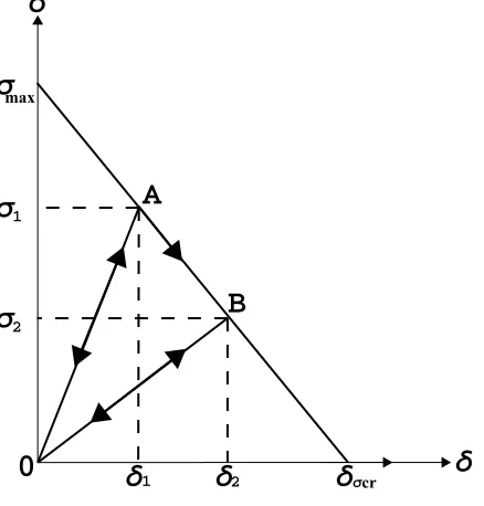
is as shown in Figure 2.4.
In the tensile case, when the normal opening displacement δσ increases
monotoni-cally, the cohesive stress (σ) are ramped down linearly as a function of δσ (Figure
2.4). The cohesive tractions reduce to zero at critical opening displacement δσ =δσcr
and remain zero upon further opening or closing. This forms a new surface and the
σ
Α
Β
δ
δ
δ
σ
σ
0
11
2 2
σ
σcr
δ
[image:35.612.200.419.30.259.2]max
Figure 2.4: Tensile cohesive relation - Ortiz-Camacho cohesive relation
However since in the laboratory earthquake experiments, an interface already exists,
the cohesive traction is completely due to cohesion between the two half spaces. Also
since no new surface is being formed and the opening is small, we can assume that the
surface is not irreversibly damaged due to the increasing crack opening displacement.
2.4.2
Reversible rate-independent cohesive model
In this section we discuss reversible rate-independent cohesive model. The
rate-independent cohesive model is similar to the Camacho-Ortiz model discussed earlier
except that it does not take into account the irreversible effects due to damage.
In the laboratory dynamic rupture experiments the damage can be considered
neg-ligible. Also since an already interface exists, new surface is not formed during the
rupture as assumed in the cohesive law in Camacho & Ortiz (1996). Hence the
open-ing and closopen-ing modes can be considered reversible and without permanent set. The
A
B
maxcr 1
0
12 2
σ
σ
σ
σ
δ
δ
δ
δ
σ
Figure 2.5: Reversible rate-independent cohesive model
the opening displacement (δn). The reversible rate-independent cohesive model is as
shown in Figure 2.5.
When the normal opening displacementδσincreases monotonically, the cohesive stress
σ is ramped down linearly as a function of δσ. The cohesive tractions reduce to zero
at critical opening displacement δσ = δσcr. When the velocity changes sign and the
interface begins to close, the cohesive is linearly ramped up to maximum strength of
Chapter 3
Validation of the developed
numerical approach
3.1
Study of Lamb’s problem on an elastic
half-space
The numerical algorithm developed has been validated using the test case of a Lamb’s
problem on an elastic half space. The problem is to determine the motion of the
sur-face of a uniform elastic half-space produced by the application of a point force pulse
varying with time like the Heaviside unit function. The original problem was
pro-posed by Lamb (1904). Closed form analytical solutions were derived for the Lamb’s
problem by Dix (1954) and Pekeris (1955).
3.1.1
Theoretical formulation of Lamb’s problem
In this section, we discuss briefly the closed form analytical solutions derived for the
Lamb’s problem (Pekeris (1955)). Let us consider a cylindrical coordinate system.
The variation of the normal force (pzz) on the surface with time is represented by the
Heaviside unit function H(t) and it’s spatial localization is such that it is everywhere
that:
2π
∞
0
pzz(r)r dr =Z (3.1)
where Z is a negative constant. The horizontal and the vertical displacements are
given to be Lamb (1904):
q =φr+χrz
w=φz+χzz−k2χ
(3.2)
where the subscripts denote partial differentiation, and the potentialsφand χsatisfy
the wave equations for educational and equivoluminal motion respectively:
∇2φ−h2φ= 0
∇2χ−k2χ= 0 (3.3)
where h2 = pc22 p, k
2 = p2
c2s, c
2
s = μρ, c2p = λ+2ρμ = 3c2s. cp represents the p-wave speed,
cs represents the s-wave speed, pdenotes the ∂t∂. λ and μ are the elastic constants of
the medium.
The surface being traction free, both normal and shear stresses reduce to zero. The
shear stress prz and the normal stress pzz are given by
prz =μ
∂
∂t 2φz+ 2χzz −k
2χ = 0
pzz =λh2φ+ 2μ
φzz+χzz−k2χz
= 0
(3.4)
The actual vertical displacement, w(r, z, t) can be obtained by performing the
inte-gration over the Bromwich contour.
w(r, z, t) = 1 2πi
a+i∞
a−i∞
ept p
w(r, z, t)dp (3.5)
expression for the vertical displacement in the case of a surface source to be given by
the integral
w(p) = Zk
2
2πμ
∞
0
J0(ξr)ξα2ξ2+k22−4k2ξ2αβ −1
dξ (3.6)
where α= (ξ2+h2)
1 2
k and β =
(ξ2+k2)12
k
A closed form solution has been derived for rocks (Poisson’ ratio (ν) = 0.25) for the
3-D case by Pekeris (1955). The expressions for the vertical displacement (w(x1, t)) of the interface forν = 0.25, assuming a traction-free boundary, are given to be:
w(x1, t) =
⎧ ⎪ ⎪ ⎪ ⎪ ⎪ ⎪ ⎪ ⎪ ⎪ ⎪ ⎪ ⎪ ⎪ ⎪ ⎪ ⎪ ⎪ ⎪ ⎪ ⎪ ⎨ ⎪ ⎪ ⎪ ⎪ ⎪ ⎪ ⎪ ⎪ ⎪ ⎪ ⎪ ⎪ ⎪ ⎪ ⎪ ⎪ ⎪ ⎪ ⎪ ⎪ ⎩
0 if τ <1/√3
− Z
32πμx1
6− √√3
τ2−14 −
√
3√3+5
3 4+
√
3 4 −τ2
+ √
3√3−5
√
3 4 −34+τ2
if 1/√3< τ <1
− Z
16πμx1
6−
√
3√3+5
3 4+
√
3 4 −τ2
if 1< τ < 123 +√3
− 3Z
8πμx1 if τ >
1 2
3 +√3
(3.7)
whereτ =cst/x1 is the reduced time andx1 is the distance to the point of application of the force.
3.1.2
Numerical investigation of Lamb’s problem
The spectral boundary integral algorithm developed has been tested using the Lamb’s
problem of step loading on a half space. In addition to the fact that it allows direct
to visualize the distinctive effects of dilatational, shear and Rayleigh waves.
The numerical simulation was performed on a square domain [0, X] by [0, X] using
a 600 by 600 spatial discretization, so that Δx1 = Δx3 = X/600, and a value of
β = csΔt/Δx1 =csΔt/Δx3 = 0.25. The point load was applied at the center of the square by assigning τ0 =P/Δx1Δx3 at that node and τ0 = 0 elsewhere.
0 0.5 1 1.5 2
−0.2 −0.15 −0.1 −0.05 0 0.05 0.1 0.15 0.2
c
st/L
δ 2
/
Δ
X
Displacement vs. Time
[image:40.612.173.445.180.446.2]Numerical Analytical
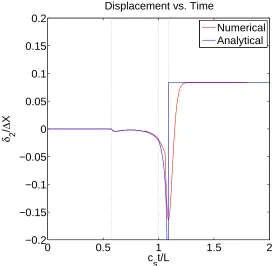
Figure 3.1: Evolution of displacement normal to the traction-free surface at a point located at a distance L from the point of application of load. Dotted lines denote the arrival times of dilatational, shear and Rayleigh waves.
A direct comparison is presented in Figure 3.1 and it illustrates the evolution of the
displacement component u2 normal to the free surface at a distance of 64 elements away from the point of application of force. We can observe a good agreement
be-tween the two solutions. The numerical scheme is also able to capture the arrival
of dilatational, shear and Rayleigh waves. The solution shows spurious numerical
oscillations of small amplitude prior to and at the arrival of the dilatational wave.
at the arrival of the Rayleigh wave, the numerical computed crack opening smoothes
out and experiences a Gibbs effect before settling down to the final constant value.
This effect is attributed to the discrete Fourier representation of the fields which are
unable to capture a discontinuity.
z/X
Figure 3.2: Displacement field on the surface of the half space after 200 time steps, showing the concentric waves expanding from the point of application of point load
Figure 3.2 shows the three-dimensional view of the displacement field after 200 time
steps. It clearly shows the dilatational precursor which creates the small
displace-ment in the direction opposite to that of the applied force, the singular Rayleigh wave
expanding radially from the point of application of force and the 1/rsingularity after
the passage of various waves.
In summary, we find that the numerical results match the theoretical closed-form
3.2
Propagating mode-I crack in a plate
There are four length scales in dynamic rupture simulations.
1. The macroscopic scale Lcharacterizes the geometry of the body.
2. The critical crack size (2Lc) is the length of the crack at equilibrium. Upon any
further loading, the crack becomes unstable and grows rapidly.
3. The cohesive zone length (lz) is the measure of the length over which the cohesive
constitutive relation plays a role.
4. The mesh size Δx provides a non-physical length scale. It is necessary that Δx
is smaller than all the physical scales 1-3 for the mesh to provide an accurate
resolution.
3.2.1
Critical crack length
In this section we review the procedure adopted by Griffith (1920) to computing the
critical crack length by considering a body with an internal crack and which is
sub-jected to external loads as shown in Figure 3.3.
According to the law of conservation of energy, the work performed per unit time by
the applied loads ( ˙W) must be equal to the rates of change of the internal elastic
energy ( ˙UE), plastic energy ( ˙UP), kinetic energy ( ˙K) of the body, and the energy per
unit time ( ˙Γ) spent in increasing the crack area.
( ˙W) = ( ˙UE) + ( ˙UP) + ( ˙K) + ( ˙Γ) (3.8)
where a dot over the letter refers to differentiation with respect to time.
Since all the changes with respect to time are caused by changes in crack size, we
have
∂ ∂t =
∂ ∂A
∂A ∂t = ˙A
∂