WRL 93 6 pdf

WRL

Research Report 93/6

Limits of

Instruction-Level

Parallelism

The Western Research Laboratory (WRL) is a computer systems research group that was founded by Digital Equipment Corporation in 1982. Our focus is computer science research relevant to the design and application of high performance scientific computers. We test our ideas by designing, building, and using real systems. The systems we build are research prototypes; they are not intended to become products.

There two other research laboratories located in Palo Alto, the Network Systems Laboratory (NSL) and the Systems Research Center (SRC). Other Digital research groups are located in Paris (PRL) and in Cambridge, Massachusetts (CRL).

Our research is directed towards mainstream high-performance computer systems. Our prototypes are intended to foreshadow the future computing environments used by many Digital customers. The long-term goal of WRL is to aid and accelerate the development of high-performance uni- and multi-processors. The research projects within WRL will address various aspects of high-performance computing.

We believe that significant advances in computer systems do not come from any single technological advance. Technologies, both hardware and software, do not all advance at the same pace. System design is the art of composing systems which use each level of technology in an appropriate balance. A major advance in overall system performance will require reexamination of all aspects of the system.

We do work in the design, fabrication and packaging of hardware; language processing and scaling issues in system software design; and the exploration of new applications areas that are opening up with the advent of higher performance systems. Researchers at WRL cooperate closely and move freely among the various levels of system design. This allows us to explore a wide range of tradeoffs to meet system goals.

We publish the results of our work in a variety of journals, conferences, research reports, and technical notes. This document is a research report. Research reports are normally accounts of completed research and may include material from earlier technical notes. We use technical notes for rapid distribution of technical material; usually this represents research in progress.

Research reports and technical notes may be ordered from us. You may mail your order to:

Technical Report Distribution

DEC Western Research Laboratory, WRL-2 250 University Avenue

Palo Alto, California 94301 USA

Reports and notes may also be ordered by electronic mail. Use one of the following addresses:

Digital E-net: DECWRL::WRL-TECHREPORTS

Internet: [email protected]

UUCP: decwrl!wrl-techreports

David W. Wall

Abstract

Growing interest in ambitious multiple-issue machines and heavily-pipelined machines requires a careful examination of how much instruction-level parallelism exists in typical programs. Such an examination is compli-cated by the wide variety of hardware and software techniques for increasing the parallelism that can be exploited, including branch prediction, register renaming, and alias analysis. By performing simulations based on instruc-tion traces, we can model techniques at the limits of feasibility and even beyond. This paper presents the results of simulations of 18 different test programs under 375 different models of available parallelism analysis.

Three years ago I published some preliminary results of a simulation-based study of instruction-level parallelism [Wall91]. It took advantage of a fast instruction-instruction-level simulator and a computing environment in which I could use three or four dozen machines with performance in the 20-30 MIPS range every night for many weeks. But the space of parallelism techniques to be explored is very large, and that study only scratched the surface.

The report you are reading now is an attempt to fill some of the cracks, both by simulating more intermediate models and by considering a few ideas the original study did not consider. I believe it is by far the most extensive study of its kind, requiring almost three machine-years and simulating in excess of 1 trillion instructions.

The original paper generated many different opinions1_{. Some looked at the high parallelism}

available from very ambitious (some might say unrealistic) models and proclaimed the millen-nium. My own opinion was pessimistic: I looked at how many different things you have to get right, including things this study doesn’t address at all, and despaired. Since then I have moderated that opinion somewhat, but I still consider the negative results of this study to be at least as important as the positive.

This study produced far too many numbers to present them all in the text and graphs, so the complete results are available only in the appendix. I have tried not to editorialize in the selection of which results to present in detail, but a careful study of the numbers in the appendix may well reward the obsessive reader.

LIMITS OFINSTRUCTION-LEVELPARALLELISM

1

Introduction

In recent years there has been an explosion of interest in multiple-issue machines. These are designed to exploit, usually with compiler assistance, the parallelism that programs exhibit at the instruction level. Figure 1 shows an example of this parallelism. The code fragment in 1(a) consists of three instructions that can be executed at the same time, because they do not depend on each other’s results. The code fragment in 1(b) does have dependencies, and so cannot be executed in parallel. In each case, the parallelism is the number of instructions divided by the number of cycles required.

r1 := 0[r9] r1 := 0[r9]

r2 := 17 r2 := r1 + 17

4[r3] := r6 4[r2] := r6

(a) parallelism=3 (b) parallelism=1

Figure 1: Instruction-level parallelism (and lack thereof)

Architectures have been proposed to take advantage of this kind of parallelism. A superscalar machine [AC87] is one that can issue multiple independent instructions in the same cycle. A superpipelined machine [JW89] issues one instruction per cycle, but the cycle time is much smaller than the typical instruction latency. A VLIW machine [NF84] is like a superscalar machine, except the parallel instructions must be explicitly packed by the compiler into very long instruction words.

Most “ordinary” pipelined machines already have some degree of parallelism, if they have operations with multi-cycle latencies; while these instructions work, shorter unrelated instructions can be performed. We can compute the degree of parallelism by multiplying the latency of each operation by its relative dynamic frequency in typical programs. The latencies of loads, delayed branches, and floating-point instructions give the DECstation2 5000, for example, a parallelism equal to about 1.5.

A multiple-issue machine has a hardware cost beyond that of a scalar machine of equivalent technology. This cost may be small or large, depending on how aggressively the machine pursues instruction-level parallelism. In any case, whether a particular approach is feasible depends on its cost and the parallelism that can be obtained from it.

But how much parallelism is there to exploit? This is a question about programs rather than about machines. We can build a machine with any amount of instruction-level parallelism we choose. But all of that parallelism would go unused if, for example, we learned that programs consisted of linear sequences of instructions, each dependent on its predecessor’s result. Real programs are not that bad, as Figure 1(a) illustrates. How much parallelism we can find in a program, however, is limited by how hard we are willing to work to find it.

A number of studies [JW89, SJH89, TF70] dating back 20 years show that parallelism within a basic block rarely exceeds 3 or 4 on the average. This is unsurprising: basic blocks are typically around 10 instructions long, leaving little scope for a lot of parallelism. At the other extreme is a study by Nicolau and Fisher [NF84] that finds average parallelism as high as 1000, by considering highly parallel numeric programs and simulating a machine with unlimited hardware parallelism and an omniscient scheduler.

There is a lot of space between 3 and 1000, and a lot of space between analysis that looks only within basic blocks and analysis that assumes an omniscient scheduler. Moreover, this space is multi-dimensional, because parallelism analysis consists of an ever-growing body of complementary techniques. The payoff of one choice depends strongly on its context in the other choices made. The purpose of this study is to explore that multi-dimensional space, and provide some insight about the importance of different techniques in different contexts. We looked at the parallelism of 18 different programs at more than 350 points in this space.

The next section describes the capabilities of our simulation system and discusses the various parallelism-enhancing techniques it can model. This is followed by a long section looking at some of the results; a complete table of the results is given in an appendix. Another appendix gives details of our implementation of these techniques.

2

Our experimental framework

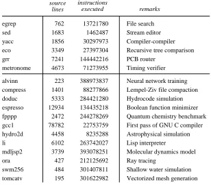
We studied the instruction-level parallelism of eighteen test programs. Twelve of these were taken from the SPEC92 suite; three are common utility programs, and three are CAD tools written at WRL. These programs are shown in Figure 2. The SPEC benchmarks were run on accompanying test data, but the data was usually an official “short” data set rather than the reference data set, and in two cases we modified the source to decrease the iteration count of the outer loop. Appendix 2 contains the details of the modifications and data sets. The programs were compiled for a DECStation 5000, which has a MIPS R30003 processor. The Mips version 1.31 compilers were used.

Like most studies of instruction-level parallelism, we used oracle-driven trace-based simu-lation. We begin by obtaining a trace of the instructions executed.4 _{This trace also includes the}

data addresses referenced and the results of branches and jumps. A greedy scheduling algorithm, guided by a configurable oracle, packs these instructions into a sequence of pending cycles. The resulting sequence of cycles represents a hypothetical execution of the program on some multiple-issue machine. Dividing the number of instructions executed by the number of cycles required gives the average parallelism.

LIMITS OFINSTRUCTION-LEVELPARALLELISM

sed 1683 1462487 Stream editor egrep 762 13721780 File search

yacc 1856 30297973 Compiler-compiler

metronome 4673 71273955 Timing verifier grr 7241 144442216 PCB router

eco 3349 27397304 Recursive tree comparison

gcc1 78782 22753759 First pass of GNU C compiler espresso 12934 134435218 Boolean function minimizer

li 6102 263742027 Lisp interpreter

fpppp 2472 244278269 Quantum chemistry benchmark doduc 5333 284421280 Hydrocode simulation

tomcatv 195 301622982 Vectorized mesh generation source

lines

instructions

executed remarks

hydro2d 4458 8235288 Astrophysical simulation compress 1401 88277866 Lempel-Ziv file compaction

ora 427 212125692 Ray tracing

swm256 484 301407811 Shallow water simulation alvinn 223 388973837 Neural network training

mdljsp2 3739 393078251 Molecular dynamics model

Figure 2: The eighteen test programs

Figure 3 illustrates the different kinds of dependencies. Some dependencies are real, reflecting the true flow of the computation. Others are false dependencies, accidents of the code generation or our lack of precise knowledge about the flow of data. Two instructions have a true data dependency if the result of the first is an operand of the second. Two instructions have an anti-dependency if the first uses the old value in some location and the second sets that location to a new value. Similarly, two instructions have an output dependency if they both assign a value to the same location. Finally, there is a control dependency between a branch and an instruction whose execution is conditional on it.

The oracle uses an actual program trace to make its decisions. This lets it “predict the future,” basing its scheduling decisions on its foreknowledge of whether a particular branch will be taken or not, or whether a load and store refer to the same memory location. It can therefore construct an impossibly perfect schedule, constrained only by the true data dependencies between instructions, but this does not provide much insight into how a real machine would perform. It is more interesting to hobble the oracle in ways that approximate the capabilities of a real machine and a real compiler system.

(a) true data dependency

r1 := 20[r4]

...

r2 := r1 + 1

(b) anti-dependency

r2 := r1 + r4

r1 := r17 - 1

...

(c) output dependency

r1 := r2 * r3

r1 := 0[r7]

...

(d) control dependency

if r17 = 0 goto L ...

r1 := r2 + r3 ...

L:

Figure 3: Dependencies

2.1

Register renaming

Anti-dependencies and output dependencies on registers are often accidents of the compiler’s register allocation technique. In Figures 3(b) and 3(c), using a different register for the new value in the second instruction would remove the dependency. Register allocation that is integrated with the compiler’s instruction scheduler [BEH91, GH88] could eliminate many of these. Current compilers often do not exploit this, preferring instead to reuse registers as often as possible so that the number of registers needed is minimized.

An alternative is the hardware solution of register renaming, in which the hardware imposes a level of indirection between the register number appearing in the instruction and the actual register used. Each time an instruction sets a register, the hardware selects an actual register to use for as long as that value is needed. In a sense the hardware does the register allocation dynamically. Register renaming has the additional advantage of allowing the hardware to include more registers than will fit in the instruction format, further reducing false dependencies.

LIMITS OFINSTRUCTION-LEVELPARALLELISM

2.2

Alias analysis

Like registers, memory locations can also carry true and false dependencies. We make the assumption that renaming of memory locations is not an option, for two reasons. First, memory is so much larger than a register file that renaming could be quite expensive. More important, though, is that memory locations tend to be used quite differently from registers. Putting a value in some memory location normally has some meaning in the logic of the program; memory is not just a scratchpad to the extent that the registers are.

Moreover, it is hard enough just telling when a memory-carried dependency exists. The registers used by an instruction are manifest in the instruction itself, while the memory location used is not manifest and in fact may be different for different executions of the instruction. A multiple-issue machine may therefore be forced to assume that a dependency exists even when it might not. This is the aliasing problem: telling whether two memory references access the same memory location.

Hardware mechanisms such as squashable loads have been suggested to help cope with the aliasing problem. The more conventional approach is for the compiler to perform alias analysis, using its knowledge of the semantics of the language and the program to rule out dependencies whenever it can.

Our system provides four levels of alias analysis. We can assume perfect alias analysis, in which we look at the actual memory address referenced by a load or store; a store conflicts with a load or store only if they access the same location. We can also assume no alias analysis, so that a store always conflicts with a load or store. Between these two extremes would be alias analysis as a smart vectorizing compiler might do it. We don’t have such a compiler, but we have implemented two intermediate schemes that may give us some insight.

One intermediate scheme is alias by instruction inspection. This is a common technique in compile-time instruction-level code schedulers. We look at the two instructions to see if it is obvious that they are independent; the two ways this might happen are shown in Figure 4.

r1 := 0[r9] r1 := 0[fp] 4[r9] := r2 0[gp] := r2

(a) (b)

Figure 4: Alias analysis by inspection

The two instructions in 4(a) cannot conflict, because they use the same base register but different displacements. The two instructions in 4(b) cannot conflict, because their base registers show that one refers to the stack and the other to the global data area.

The idea behind our model of alias analysis by compiler is that references outside the heap can often be resolved by the compiler, by doing dataflow and dependency analysis over loops and arrays, whereas heap references are often less tractable. Neither of these assumptions is particularly defensible. Many languages allow pointers into the stack and global areas, rendering them as difficult as the heap. Practical considerations such as separate compilation may also keep us from analyzing non-heap references perfectly. On the other side, even heap references may not be as hopeless as this model assumes [CWZ90, HHN92, JM82, LH88]. Nevertheless, our range of four alternatives should provide some intuition about the effects of alias analysis on instruction-level parallelism.

2.3

Branch prediction

Parallelism within a basic block is usually quite limited, mainly because basic blocks are usually quite small. The approach of speculative execution tries to mitigate this by scheduling instructions across branches. This is hard because we don’t know which way future branches will go and therefore which path to select instructions from. Worse, most branches go each way part of the time, so a branch may be followed by two possible code paths. We can move instructions from either path to a point before the branch only if those instructions will do no harm (or if the harm can be undone) when we take the other path. This may involve maintaining shadow registers, whose values are not committed until we are sure we have correctly predicted the branch. It may involve being selective about the instructions we choose: we may not be willing to execute memory stores speculatively, for example, or instructions that can raise exceptions. Some of this may be put partly under compiler control by designing an instruction set with explicitly squashable instructions. Each squashable instruction would be tied explicitly to a condition evaluated in another instruction, and would be squashed by the hardware if the condition turns out to be false. If the compiler schedules instructions speculatively, it may even have to insert code to undo its effects at the entry to the other path.

The most common approach to speculative execution uses branch prediction. The hardware or the software predicts which way a given branch will most likely go, and speculatively schedules instructions from that path.

LIMITS OFINSTRUCTION-LEVELPARALLELISM

4 6 8 10 12 14 16 18 0.5

1

0.55 0.6 0.65 0.7 0.75 0.8 0.85 0.9 0.95

prediction success rate

tomcatv swm256 alvinn sed doduc yacc mdljsp2 fpppp met hydro2d eco gcc1 egrep compress li espresso ora grr

harmonic mean

16 64 256 1K 4K 16K 64K 256K

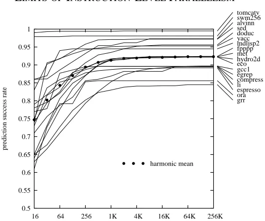
Figure 5: Fraction of branches predicted correctly using two-bit counter prediction, as a function of the total number of bits in the predictor

which tells for each branch what fraction of its executions it was taken. Like any profile, a branch profile is obtained by inserting counting code into a test program, to keep track of how many times each branch goes each way. We use a branch profile by seeing which way a given branch goes most often, and scheduling instructions from that path. If there is some expense in undoing speculative execution when the branch goes the other way, we might impose a threshold so that we don’t move instructions across a branch that is executed only 51% of the time.

Recent studies have explored more sophisticated hardware prediction using branch histo-ries [PSR92, YP92, YP93]. These approaches maintain tables relating the recent history of the branch (or of branches in the program as a whole) to the likely next outcome of the branch. These approaches do quite poorly with small tables, but unlike the two-bit counter schemes they can benefit from much larger predictors.

An example is the local-history predictor [YP92]. It maintains a table ofn-bit shift registers,

indexed by the branch address as above. When the branch is taken, a 1 is shifted into the table entry for that branch; otherwise a 0 is shifted in. To predict a branch, we take itsn-bit history

and use it as an index into a table of 2n

2-bit counters like those in the simple counter scheme described above. If the counter is 2 or 3, we predict taken; otherwise we predict not taken. If the prediction proves correct, we increment the counter; otherwise we decrement it. The local-history predictor works well on branches that display a regular pattern of small period.

Sometimes the behavior of one branch is correlated with the behavior of another. A global-history predictor [YP92] tries to exploit this effect. It replaces the table of shift registers with a single shift register that records the outcome of thenmost recently executed branches, and uses

4 6 8 10 12 14 16 18 20 0.7

1

0.75 0.8 0.85 0.9 0.95

prediction success rate

counter ctr/gsh loc/gsh

16 64 256 1K 4K 16K 64K 256K 1M

Figure 6: Fraction of branches predicted correctly by three different prediction schemes, as a function of the total number of bits in the predictor

An interesting variation is the gshare predictor [McF93], which uses the identity of the branch as well as the recent global history. Instead of indexing the array of counters with just the global history register, the gshare predictor computes thexorof the global history and branch address. McFarling [McF93] got even better results by using a table of two-bit counters to dynamically choose between two different schemes running in competition. Each predictor makes its prediction as usual, and the branch address is used to select another 2-bit counter from a selector table; if the selector value is 2 or 3, the first prediction is used; otherwise the second is used. When the branch outcome is known, the selector is incremented or decremented if exactly one predictor was correct. This approach lets the two predictors compete for authority over a given branch, and awards the authority to the predictor that has recently been correct more often. McFarling found that combined predictors did not work as well as simpler schemes when the predictor size was small, but did quite well indeed when large.

LIMITS OFINSTRUCTION-LEVELPARALLELISM

ctrs ctrs ctrs ctrs ctr/gsh loc/gsh loc/gsh prof sign taken

4b 8b 16b 64b 2kb 16kb 152k

egrep 0.75 0.78 0.77 0.87 0.90 0.95 0.98 0.90 0.65 0.80

sed 0.75 0.81 0.74 0.92 0.97 0.98 0.98 0.97 0.42 0.71

yacc 0.74 0.80 0.83 0.92 0.96 0.97 0.98 0.92 0.60 0.73

eco 0.57 0.61 0.64 0.77 0.95 0.97 0.98 0.91 0.46 0.61

grr 0.58 0.60 0.65 0.73 0.89 0.92 0.94 0.78 0.54 0.51

metronome 0.70 0.73 0.73 0.83 0.95 0.97 0.98 0.91 0.61 0.54

alvinn 0.86 0.84 0.86 0.89 0.98 1.00 1.00 0.97 0.85 0.84

compress 0.64 0.73 0.75 0.84 0.89 0.90 0.90 0.86 0.69 0.55

doduc 0.54 0.53 0.74 0.84 0.94 0.96 0.97 0.95 0.76 0.45

espresso 0.72 0.73 0.78 0.82 0.93 0.95 0.96 0.86 0.62 0.63

fpppp 0.62 0.59 0.65 0.81 0.93 0.97 0.98 0.86 0.46 0.58

gcc1 0.59 0.61 0.63 0.70 0.87 0.91 0.94 0.88 0.50 0.57

hydro2d 0.69 0.75 0.79 0.85 0.94 0.96 0.97 0.91 0.51 0.68

li 0.61 0.69 0.71 0.77 0.95 0.96 0.98 0.88 0.54 0.46

mdljsp2 0.82 0.84 0.86 0.94 0.95 0.96 0.97 0.92 0.31 0.83

ora 0.48 0.55 0.61 0.79 0.91 0.98 0.99 0.87 0.54 0.51

swm256 0.97 0.97 0.98 0.98 1.00 1.00 1.00 0.98 0.98 0.91

tomcatv 0.99 0.99 0.99 0.99 1.00 1.00 1.00 0.99 0.62 0.99

hmean 0.68 0.71 0.75 0.84 0.94 0.96 0.97 0.90 0.55 0.63

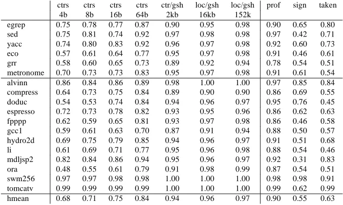
Figure 7: Success rates of different branch prediction techniques

the three hardware prediction schemes shown in Figure 6 with any predictor size. We can also assume three kinds of static branch prediction: profiled branch prediction, in which we predict that the branch will go the way it went most frequently in a profiled previous run; signed branch prediction, in which we predict that a backward branch will be taken but a forward branch will not, and taken branch prediction, in which we predict that every branch will always be taken. And finally, we can assume that no branch prediction occurs; this is the same as assuming that every branch is predicted wrong.

Figure 7 shows the actual success rate of prediction using different sizes of tables. It also shows the success rates for the three kinds of static prediction. Profiled prediction routinely beats 64-bit counter-based prediction, but it cannot compete with the larger, more advanced techniques. Signed or taken prediction do quite poorly, about as well as the smallest of dynamic tables; of the two, taken prediction is slightly the better. Signed prediction, however, lends itself better to the compiler technique of moving little-used pieces of conditionally executed code out of the normal code stream, improving program locality and thereby the cache performance.

The effect of branch prediction on scheduling is easy to state. Correctly predicted branches have no effect on scheduling (except for register dependencies involving their operands). Instruc-tions appearing later than a mispredicted branch cannot be scheduled before the branch itself, since we do not know we should be scheduling them until we find out that the branch went the other way. (Of course, both the branch and the later instruction may be scheduled before instructions that precede the branch, if other dependencies permit.)

2.4

Branch fanout

Rather than try to predict the destinations of branches, we might speculatively execute instructions along both possible paths, squashing the wrong path when we know which it is. Some of our hardware parallelism capability is guaranteed to be wasted, but we will never miss out completely by blindly taking the wrong path. Unfortunately, branches happen quite often in normal code, so for large degrees of parallelism we may encounter another branch before we have resolved the previous one. Thus we cannot continue to fan out indefinitely: we will eventually use up all the machine parallelism just exploring many parallel paths, of which only one is the right one. An alternative if the branch probability is available, as from a profile, is to explore both paths if the branch probability is near 0.5 but explore the likely path when its probability is near 1.0.

Our system allows the scheduler to explore in both directions past branches. Because the scheduler is working from a trace, it cannot actually schedule instructions from the paths not taken. Since these false paths would use up hardware parallelism, we model this by assuming that there is an upper limit on the number of branches we can look past. We call this upper limit the fanout limit. In terms of our simulator scheduling, branches where we explore both paths are simply considered to be correctly predicted; their effect on the schedule is identical, though of course they use up part of the fanout limit.

In some respects fanout duplicates the benefits of branch prediction, but they can also work together to good effect. If we are using dynamic branch prediction, we explore both paths up to the fanout limit, and then explore only the predicted path beyond that point. With static branch prediction based on a profile we go still further. It is easy to implement a profiler that tells us not only which direction the branch went most often, but also the frequency with which it went that way. This lets us explore only the predicted path if its predicted probability is above some threshold, and use our limited fanout ability to explore both paths only when the probability of each is below the threshold.

2.5

Indirect-jump prediction

Most architectures have two kinds of instructions to change the flow of control. Branches are conditional and have a destination that is some specified offset from the PC. Jumps are unconditional, and may be either direct or indirect. A direct jump is one whose destination is given explicitly in the instruction, while an indirect jump is one whose destination is expressed as an address computation involving a register. In principle we can know the destination of a direct jump well in advance. The destination of an indirect jump, however, may require us to wait until the address computation is possible. Predicting the destination of an indirect jump might pay off in instruction-level parallelism.

We consider two jump prediction strategies, which can often be used simultaneously.

LIMITS OFINSTRUCTION-LEVELPARALLELISM

n-element return ring 2K-ring plusn-element table prof

1 2 4 8 16 2K 2 4 8 16 32 64

egrep 0.99 0.99 0.99 0.99 1.00 1.00 1.00 1.00 1.00 1.00 1.00 1.00 0.99

sed 0.27 0.46 0.68 0.68 0.68 0.68 0.97 0.97 0.97 0.97 0.97 0.97 0.97

yacc 0.68 0.85 0.88 0.88 0.88 0.88 0.92 0.92 0.92 0.92 0.92 0.92 0.71

eco 0.48 0.66 0.76 0.77 0.77 0.78 0.82 0.82 0.82 0.82 0.82 0.82 0.56

grr 0.69 0.84 0.92 0.95 0.95 0.95 0.98 0.98 0.98 0.98 0.98 0.98 0.65

met 0.76 0.88 0.96 0.97 0.97 0.97 0.99 0.99 0.99 0.99 0.99 0.99 0.65

alvinn 0.33 0.43 0.63 0.90 0.90 0.90 1.00 1.00 1.00 1.00 1.00 1.00 0.75

compress 1.00 1.00 1.00 1.00 1.00 1.00 1.00 1.00 1.00 1.00 1.00 1.00 1.00

doduc 0.64 0.75 0.88 0.94 0.94 0.94 0.96 0.99 0.99 0.99 1.00 1.00 0.62

espresso 0.76 0.89 0.95 0.96 0.96 0.96 1.00 1.00 1.00 1.00 1.00 1.00 0.54

fpppp 0.55 0.71 0.73 0.74 0.74 0.74 0.99 0.99 0.99 0.99 0.99 0.99 0.80

gcc1 0.46 0.61 0.71 0.74 0.74 0.74 0.81 0.82 0.82 0.83 0.83 0.84 0.60

hydro2d 0.42 0.50 0.57 0.61 0.62 0.62 0.72 0.72 0.76 0.77 0.80 0.82 0.64

li 0.44 0.57 0.72 0.81 0.84 0.86 0.91 0.91 0.93 0.93 0.93 0.93 0.69

mdljsp2 0.97 0.98 0.99 0.99 0.99 0.99 0.99 0.99 0.99 0.99 1.00 1.00 0.98

ora 0.97 1.00 1.00 1.00 1.00 1.00 1.00 1.00 1.00 1.00 1.00 1.00 0.46

swm256 0.99 0.99 0.99 0.99 0.99 0.99 1.00 1.00 1.00 1.00 1.00 1.00 0.26

tomcatv 0.41 0.48 0.59 0.63 0.63 0.63 0.71 0.71 0.77 0.78 0.85 0.85 0.72

hmean 0.56 0.69 0.80 0.84 0.84 0.85 0.92 0.92 0.93 0.93 0.94 0.95 0.63

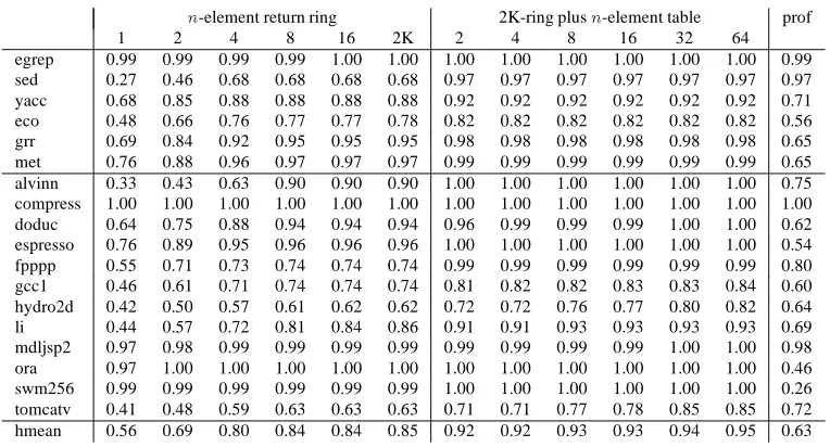
Figure 8: Success rates of different jump prediction techniques

table entry and interfering with each other.

The second strategy involves procedure returns, the most common kind of indirect jump. If the machine can distinguish returns from other indirect jumps, it can do a better job of predicting their destinations, as follows. The machine maintains a small ring buffer of return addresses. Whenever it executes a subroutine call instruction, it increments the buffer pointer and enters the return address in the buffer. A return instruction is predicted to go to the last address in this buffer, and then decrements the buffer pointer. Unless we do tail-call optimization or setjmp/longjmp, this prediction will always be right if the machine uses a big enough ring buffer. Even if it cannot distinguish returns from other indirect jumps, their predominance might make it worth predicting that any indirect jump is a return, as long as we decrement the buffer pointer only when the prediction succeeds.

Our system allows several degrees of each kind of jump prediction. We can assume that indirect jumps are perfectly predicted. We can use the cacheing prediction, in which we predict that a jump will go wherever it went last time, with a table of any size. Subroutine returns can be predicted with this table, or with their own return ring, which can also be any desired size. We can also predict returns with a return ring and leave other indirect jumps unpredicted. Finally, we can assume no jump prediction whatsoever.

As with branches, a correctly predicted jump has no effect on the scheduling. A mispredicted or unpredicted jump may be moved before earlier instructions, but no later instruction can be moved before the jump.

predict non-returns produces a substantial improvement, although the success rate does not rise much as we make the table bigger. With only an 8-element return ring and a 2-element table, we can predict more than 90% of the indirect jumps. The most-common-destination profile, in contrast, succeeds only about two thirds of the time.

2.6

Window size and cycle width

The window size is the maximum number of instructions that can appear in the pending cycles at any time. By default this is 2048 instructions. We can manage the window either discretely or continuously. With discrete windows, we fetch an entire window of instructions, schedule them into cycles, issue those cycles, and then start fresh with a new window. A missed prediction also causes us to start over with a full-size new window. With continuous windows, new instructions enter the window one at a time, and old cycles leave the window whenever the number of instructions reaches the window size. Continuous windows are the norm for the results described here, although to implement them in hardware is more difficult. Smith et al. [SJH89] assumed discrete windows.

The cycle width is the maximum number of instructions that can be scheduled in a given cycle. By default this is 64. Our greedy scheduling algorithm works well when the cycle width is large: a small proportion of cycles are completely filled. For cycle widths of 2 or 4, however, a more traditional approach [HG83, JM82] would be more realistic.

Along with cycles of a fixed finite size, we can specify that cycles are unlimited in width. In this case, there is still an effective limit imposed by the window size: if one cycle contains a window-full of instructions, it will be issued and a new cycle begun. As a final option, we therefore also allow both the cycle width and the window size to be unlimited.5

2.7

Latency

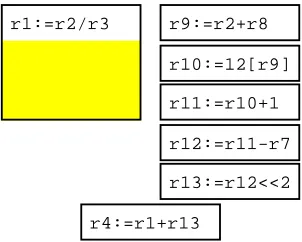
For most of our experiments we assumed that every operation had unit latency: any result computed in cycle n could be used as an operand in cycle n +1. This can obviously be

accomplished by setting the machine cycle time high enough for even the slowest of operations to finish in one cycle, but in general this is an inefficient use of the machine. A real machine is more likely to have a cycle time long enough to finish most common operations, like integer add, but let other operations (e.g. division, multiplication, floating-point operations, and memory loads) take more than one cycle to complete. If an operation in cyclet has latencyL, its result

cannot be used until cyclet+L.

LIMITS OFINSTRUCTION-LEVELPARALLELISM

(a) multi-cycle instruction is on critical path (b) multi-cycle instruction is not on critical path

r9:=r2+r8

r10:=12[r9]

r11:=r10+1

r12:=r11-r7

r13:=r12<<2

r4:=r1+r13 r1:=r2/r3

r9:=12[r1] r10:=r1+1 r1:=r2/r3

r11:=r9+r10

Figure 9: Effects of increasing latency on parallelism

model A model B model C model D model E

int add/sub, logical 1 1 1 1 1

load 1 1 2 2 3

int mult 1 2 2 3 5

int div 1 2 3 4 6

single-prec add/sub 1 2 3 4 4

single-prec mult 1 2 3 4 5

single-prec div 1 2 3 5 7

double-prec add/sub 1 2 3 4 4

double-prec mult 1 2 3 4 6

double-prec div 1 2 3 5 10

Figure 10: Operation latencies in cycles, under five latency models

by the number of cycles required. If all instructions have a latency of 1, the total latency is just the number of instructions, and the definition is the same as before. Notice that with non-unit latencies it is possible for the instruction-level parallelism to exceed the cycle width; at any given time we can be working on instructions issued in several different cycles, at different stages in the execution pipeline.

It is not obvious whether increasing the latencies of some operations will tend to increase or decrease instruction-level parallelism. Figure 9 illustrates two opposing effects. In 9(a), we have a divide instruction on the critical path; if we increase its latency we will spend several cycles working on nothing else, and the parallelism will decrease. In 9(b), in contrast, the divide is not on the critical path, and increasing its latency will increase the parallelism. Note that whether the parallelism increases or not, it is nearly certain that the time required is less, because an increase in the latency means we have decreased the cycle time.

none

perfect inspect none

perfect 64 256 none

perfect 16-addr ring, no table

2K-addr ring, 2K-addr table 16-addr ring, 8-addr table none

perfect 152Kb loc/gsh

64b counter 2Kb ctr/gsh 16Kb loc/gsh fanout 4, then 152Kb loc/gsh

Poor

Fair

Good

Great

Superb

Perfect

predict branch

analysis alias renaming

register jump

predict

Stupid

Poor

Fair

Good

Great

Superb Stupid

Perfect

Figure 11: Seven increasingly ambitious models

3

Results

LIMITS OFINSTRUCTION-LEVELPARALLELISM

701 702 703 704 705 706 707 1 64 parallelism 10 fpppp tomcatv doduc egrep swm256 hydro2d espresso gcc1 mdljsp2 grr compress sed met yacc eco li ora alvinn harmonic mean 2 3 4 5 6 7 8 20 30 40 50

Stupid Poor Fair Good Great Superb Perfect 1701 702 703 704 12 10 tomcatv fpppp swm256 hydro2d doduc met mdljsp2 li sed ora yacc espresso grr eco gcc1 egrep compress alvinn 2 3 4 5 6 7 8 Stupid Poor Fair Good

Figure 12: Parallelism under the seven models, full-scale (left) and detail (right)

3.1

Parallelism under the seven models

0 10 20 30 40 50 time (megacycles)

1 64

parallelism

10

alvinn... swm256

tomcatv

ora

mdljsp2

0 10 20 30 40 50 time (megacycles)

1 64

10

alvinn... swm256

tomcatv

ora

mdljsp2

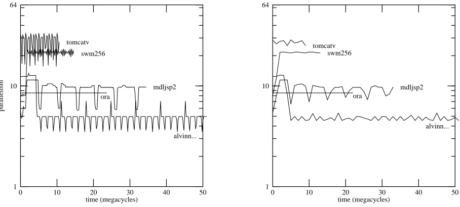
Figure 13: Parallelism under the Good model over intervals of 0.2 million cycles (left) and 1 million cycles (right)

3.2

Effects of measurement interval

We analyzed the parallelism of entire program executions because it avoided the question of what constitutes a “representative” interval. To select some smaller interval of time at random would run the risk that the interval was atypical of the program’s execution as a whole. To select a particular interval where the program is at its most parallel would be misleading and irresponsible. Figure 13 shows the parallelism under the Good model during successive intervals from the execution of some of our longer-running programs. The left-hand graph uses intervals of 200,000 cycles, the right-hand graph 1 million cycles. In each case the parallelism of an interval is computed exactly like that of a whole program: the number of instructions executed during that interval is divided by the number of cycles required.

Some of the test programs are quite stable in their parallelism. Others are quite unstable. With 200K-cycle intervals (which range from 0.7M to more than 10M instructions), the parallelism within a single program can vary widely, sometimes by a factor of three. Even 1M-cycle intervals see variation by a factor of two. The alvinn program has parallelism above 12 for 4 megacycles, at which point it drops down to less than half that; in contrast, the swm256 program starts quite low and then climbs to quite a respectable number indeed.

LIMITS OFINSTRUCTION-LEVELPARALLELISM

701 702 703 704 705 706 707 1

128

parallelism

10

100 tomcatv_doduc

fpppp egrep hydro2d swm256 espress gcc1 mdljsp2 grr compres sed met yacc eco li ora alvinn harmonic mean 2 3 4 5 6 7 8 20 30 40 50 60 70 80

Stupid Poor Fair Good Great Superb Perfect 1701 702 703 704 705 706 707 2

ratio to default

Stupid Poor Fair Good Great Superb Perfect

tomcatv doduc hydro2d fpppp espress swm256 egrep gcc1 yacc mdljsp2 grr OTHERS

Figure 14: Parallelism under the seven models with cycle width of 128 instructions (left), and the ratio of parallelism for cycles of 128 to parallelism for cycles of 64 (right)

1 2 3 4 5 6 7

1 128

parallelism

10

100 doduc_tomcatv

fpppp hydro2d egrep swm256 espresso gcc1 mdljsp2 grr compress sed met yacc eco li ora alvinn 2 3 4 5 6 7 8 20 30 40 50 60 70 80

Stupid Poor Fair Good Great Superb Perfect 1 2 3 4 5 6 7 1

2

ratio to default

Stupid Poor Fair Good Great Superb Perfect

doduc tomcatv hydro2d fpppp espress swm256 egrep gcc1 yacc mdljsp2 grr OTHERS

3.3

Effects of cycle width

Tomcatv and fpppp attain very high parallelism with even modest machine models. Their average parallelism is very close to the maximum imposed by our normal cycle width of 64 instructions; under the Great model more than half the cycles of each are completely full. This suggests that even more parallelism might be obtained by widening the cycles. Figure 14 shows what happens if we increase the maximum cycle width from 64 instructions to 128. The right-hand graph shows how the parallelism increases when we go from cycles of 64 instructions to cycles of 128. Doubling the cycle width improves four of the numeric programs appreciably under the Perfect model, and improves tomcatv by 20% even under the Great model. Most programs, however, do not benefit appreciably from such wide cycles even under the Perfect model.

Perhaps the problem is that even 128-instruction cycles are too small. If we remove the limit on cycle width altogether, we effectively make the cycle width the same as the window size, in this case 2K instructions. The results are shown in Figure 15. Parallelism in the Perfect model is a bit better than before, but outside the Perfect model we see that tomcatv is again the only benchmark to benefit significantly.

LIMITS OFINSTRUCTION-LEVELPARALLELISM

2 3 4 5 6 7 8 9 10 11 1 64 parallelism 10 fpppp tomcatv swm256 doduc espresso hydro2d met sed grr li egrep mdljsp2 gcc1 yacc ora eco compress alvinn 2 3 4 5 6 7 8 20 30 40 50

4 8 16 32 64 128 256 512 1K 2K 12 3 4 5 6 7 8 9 10 11 64

10 hydro2dtomcatv

sed met yacc li doduc compress ora eco egrep grr espresso gcc1 fpppp swm256 alvinn mdljsp2 2 3 4 5 6 7 8 20 30 40 50

4 8 16 32 64 128 256 512 1K 2K

Figure 16: Parallelism for different sizes of continuously-managed windows under the Superb model (left) and the Fair model (right)

2 3 4 5 6 7 8 9 10 11 1 64 parallelism 10 tomcatv fpppp swm256 doduc espresso hydro2d met sed li grr egrep mdljsp2 gcc1 yacc ora eco compress alvinn 2 3 4 5 6 7 8 20 30 40 50

4 8 16 32 64 128 256 512 1K 2K 2 3 4 5 6 7 8 9 10 11 1

64

10 hydro2dtomcatv

sed met yacc li doduc compress ora eco egrep grr espresso gcc1 fpppp swm256 alvinn mdljsp2 2 3 4 5 6 7 8 20 30 40 50

4 8 16 32 64 128 256 512 1K 2K

701 702 703 704 705 706 707 1 700 parallelism 10 100 swm256 hydro2d tomcatv doduc alvinn yacc egrep fpppp espresso gcc1 mdljsp2 grr compress met sed eco li ora 2 3 4 5 6 7 20 30 40 50 60 70 200 300 400 500 600

Stupid Poor Fair Good Great Superb Perfect 701 702 703 704 705 706 707 1

15

ratio to default

10

Stupid Poor Fair Good Great Superb Perfect

alvinn swm256 yacc hydro2d tomcatv doduc gcc1 espress egrep grr fpppp mdljsp2 met li eco compres OTHERS

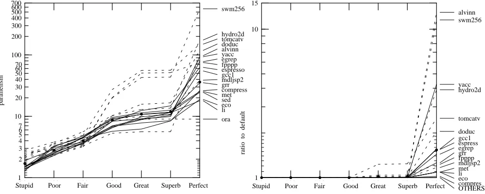
Figure 18: Parallelism under the seven models with unlimited win-dow size and cycle width (left), and the ratio of parallelism for unlim-ited windows and cycles to parallelism for 2K-instruction windows and 64-instruction cycles (right)

3.4

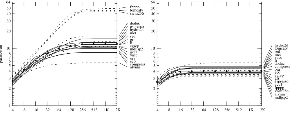
Effects of window size

Our standard models all have a window size of 2K instructions: the scheduler is allowed to keep that many instructions in pending cycles at one time. Typical superscalar hardware is unlikely to handle windows of that size, but software techniques like trace scheduling for a VLIW machine might. Figure 16 shows the effect of varying the window size from 2K instructions down to 4, for the Superb and Fair models. Under the Superb model, most programs do about as well with a 128-instruction window as with a larger one. Below that, parallelism drops off quickly. The Poor model’s limited analysis severely restricts the mobility of instructions; parallelism levels off at a window size of only 16 instructions.

LIMITS OFINSTRUCTION-LEVELPARALLELISM

Fisher’s [NF84], reaching as high as 500 for swm256 in the Perfect model. It is interesting to note that under even slightly more realistic models, the maximum parallelism drops to around 50, and the mean parallelism to around 10. The advantage of unlimited window size and cycle width outside the Perfect model shows up only on tomcatv, and even there the advantage is modest.

3.5

Effects of loop unrolling

Loop unrolling is an old compiler optimization technique that can also increase parallelism. If we unroll a loop ten times, thereby removing 90% of its branches, we effectively increase the basic block size tenfold. This larger basic block may hold parallelism that had been unavailable because of the branches or the inherent sequentiality of the loop control.

We studied the parallelism of unrolled code by manually unrolling four inner loops in three of our programs. In each case these loops constituted a sizable fraction of the original program’s total runtime. Figure 19 displays some details.

Alvinn has two inner loops, the first of which is an accumulator loop: each iteration computes a value on which no other iteration depends, but these values are successively added into a single accumulator variable. To parallelize this loop we duplicated the loop bodyntimes (withi

successively replaced byi +1,i +2, and so on wherever it occurred), collapsed thenassignments to

the accumulator into a single assignment, and then restructured the resulting large right-hand-side into a balanced tree expression.

alvinn

input_hidden hidden_input

line 109 of backprop.c line 192 of backprop.c

accumulator independent

39.5% 39.5% swm256

tomcatv

CALC2 main

line 325 of swm256.f

line 86 of tomcatv.f

14 14 independent

independent

62 258

37.8% 67.6% procedure loop location type of loop instrs % of execution

Figure 19: Four unrolled loops

The remaining three loops are perfectly parallelizable: each iteration is completely indepen-dent of the rest. We unrolled these in two different ways. In the first, we simply duplicated the loop body n times (replacing i by i+1, i+2, and so on). In the second, we duplicated the

loop bodyntimes as before, changed all assignments to array members into assignments to local

for i := 1 to N do

accum := accum + f(i); end

for i := 1 to N by 4 do accum := accum

+ ( ( f(i) + f(i+1)) + (f(i+2) + f(i+3)) );

end

for i := 1 to N do a[i] := f(i); b[i] := g(i); end

for i := 1 to N by 4 do a[i] := f(i); b[i] := g(i); a[i+1] := f(i+1); b[i+1] := g(i+1); a[i+2] := f(i+2); b[i+2] := g(i+2); a[i+3] := f(i+3); b[i+3] := g(i+3); end

for i := 1 to N by 4 do a00 := f(i);

b00 := g(i); a01 := f(i+1); b01 := g(i+1); a02 := f(i+2); b02 := g(i+2); a03 := f(i+3); b03 := g(i+3); a[i] := a00; b[i] := b00; a[i+1] := a01; b[i+1] := b01; a[i+2] := a02; b[i+2] := b02; a[i+3] := a03; b[i+3] := b03; end

Accum loop

for sophisticated models

for simple models

Figure 20: Three techniques for loop unrolling

of successive iterations. On the other hand, leaving the stores in place means that the lifetimes of computed values are shorter, allowing the compiler to do a better job of register allocation: moving the stores to the end of the loop means the compiler is more likely to start using memory locations as temporaries, which removes these values from the control of the register renaming facility available in the smarter models.

LIMITS OFINSTRUCTION-LEVELPARALLELISM

701 702 703 704 705 1

64

parallelism

10

tom-perf swm-perf alv-perf

tom-good swm-good alv-good

tom-stup swm-stup alv-stup 2

3 4 5 6 7 8 20 30 40 50

U0 U2 U4 U8 U16

Figure 21: Effects of loop unrolling

effect decreased as the unrolling factor increased. It made little difference in the other cases, and even hurt the parallelism in several instances. This difference is probably because the inner loop of alvinn is quite short, so it can be replicated several times without creating great register pressure or otherwise giving the compiler too many balls to juggle.

Moreover, it is quite possible for parallelism to go down while performance goes up. The rolled loop can do the loop bookkeeping instructions in parallel with the meat of the loop body, but an unrolled loop gets rid of at least half of that bookkeeping. Unless the unrolling creates new opportunities for parallelism (which is of course the point) this will cause the net parallelism to decrease.

Loop unrolling is a good way to increase the available parallelism, but it is not a silver bullet.

3.6

Effects of branch prediction

We saw earlier that new techniques of dynamic history-based branch prediction allow us to benefit from quite large branch predictor, giving success rates that are still improving slightly even when we are using a 1-megabit predictor. It is natural to ask how much this affects the instruction-level parallelism. Figure 22 answers this question for the Fair and Great models. The Fair model is relatively insensitive to the size of the predictor, though even a tiny 4-bit predictor improves the mean parallelism by 50%. A tiny 4-bit table doubles the parallelism under the Great model, and increasing that to a huge quarter-megabit table more than doubles it again.

0 2 4 6 8 10 12 14 16 18 1

64

parallelism

10 hydro2dsed

tomcatv met yacc li egrep doduc compress ora eco grr gcc1 espresso fpppp swm256 alvinn mdljsp2 2 3 4 5 6 7 8 20 30 40 50

0 4 16 64 256 1K 4K 16K 64K 256K 10 2 4 6 8 10 12 14 16 18 64 10 fpppp tomcatv swm256 doduc hydro2d espresso met sed li mdljsp2 egrep yacc ora grr gcc1 eco compress alvinn 2 3 4 5 6 7 8 20 30 40 50

0 4 16 64 256 1K 4K 16K 64K 256K

Figure 22: Parallelism for different sizes of dynamic branch-prediction table under the Fair model (left) and the Great model (right)

2 4 6 8 10 12 14 1

64

parallelism

10 hydro2dsed

tomcatv met yacc li egrep doduc compress ora eco grr gcc1 espresso fpppp swm256 alvinn mdljsp2 2 3 4 5 6 7 8 20 30 40 50

4 16 64 256 1K 4K 16K 12 4 6 8 10 12 14 64 10 fpppp tomcatv swm256 doduc hydro2d espresso met sed li mdljsp2 egrep yacc ora grr gcc1 eco compress alvinn 2 3 4 5 6 7 8 20 30 40 50

4 16 64 256 1K 4K 16K

instruc-LIMITS OFINSTRUCTION-LEVELPARALLELISM

701 702 703 704 705 1 64 parallelism 10 tomcatv fpppp swm256 doduc mdljsp2 hydro2d met espresso ora li sed grr gcc1 compress yacc eco egrep alvinn 2 3 4 5 6 7 8 20 30 40 50

B0 0 B22 B44 B66 B88 1701 702 703 704 705 64 10 fpppp tomcatv swm256 doduc espresso hydro2d met grr sed egrep li mdljsp2 gcc1 yacc compress ora eco alvinn 2 3 4 5 6 7 8 20 30 40 50 B0 0 B22 B44 B66 B88

Figure 24: Parallelism for the Great model with different levels of fanout scheduling across conditional branches, with no branch prediction (left) and with branch prediction (right) after fanout is exhausted

701 702 703 704 705 1 64 parallelism 10 hydro2d sed compress tomcatv met egrep yacc li doduc ora grr gcc1 eco espresso fpppp swm256 mdljsp2 alvinn 2 3 4 5 6 7 8 20 30 40 50

B0 0 B22 B44 B66 B88 1701 702 703 704 705 64 10 hydro2d sed compress yacc tomcatv met li egrep doduc ora grr gcc1 eco espresso fpppp swm256 mdljsp2 alvinn 2 3 4 5 6 7 8 20 30 40 50 B0 0 B22 B44 B66 B88

ex-the average number of instructions executed between mispredicted branches. Figure 23 shows these results. These three numeric programs still stand out as anomalies; evidently there is more involved in their parallelism than the infrequency and predictability of their branches.

3.7

Effects of fanout

Figures 24 and 25 show the effects of adding various levels of fanout to the Great and Fair models. The left-hand graphs assume that we look along both paths out of the next few conditional branches, up to the fanout limit, but that we do not look past branches beyond that point. The right-hand graphs assume that after we reach the fanout limit we use dynamic prediction (at the Great or Fair level) to look for instructions from the one predicted path to schedule. In each graph the leftmost point represents no fanout at all. We can see that when fanout is followed by good branch prediction, the fanout does not buy us much. Without branch prediction, on the other hand, even modest amounts of fanout are quite rewarding: adding fanout across 4 branches to the Fair model is about as good as adding Fair branch prediction.

Fisher [Fis91] has proposed using fanout in conjunction with profiled branch prediction. In this scheme they are both under software control: the profile gives us information that helps us to decide whether to explore a given branch using the fanout capability or using a prediction. This is possible because a profile can easily record not just which way a branch most often goes, but also how often it does so. Fisher combines this profile information with static scheduling information about the payoff of scheduling each instruction early on the assumption that the branch goes in that direction.

Our traces do not have the payoff information Fisher uses, but we can investigate a simpler variation of the idea. We pick some threshold to partition the branches into two classes: those we predict because they are very likely to go one way in particular and those at which we fan out because they are not. We will call this scheme profile-guided integrated prediction and fanout.

We modified the Perfect model to do profile-guided integrated prediction and fanout. Figure 26 shows the parallelism for different threshold levels. Setting the threshold too low means that we use the profile to predict most branches and rarely benefit from fanout: a threshold of 0.5 causes all branches to be predicted with no use of fanout at all. Setting the threshold too high means that you fan out even on branches that nearly always go one way, wasting the hardware parallelism that fanout enables. Even a very high threshold is better than none, however; some branches really do go the same way all or essentially all of the time. The benefit is not very sensitive to the threshold we use: between 0.75 and 0.95 most of the curves are quite flat; this holds as well if we do the same experiment using the Great model or the Fair model. The best threshold seems to be around 0.92.

LIMITS OFINSTRUCTION-LEVELPARALLELISM

0.5 0.6 0.7 0.8 0.9 1 1 64 parallelism 10 fpppp tomcatv swm256 doduc mdljsp2 hydro2d sed li met gcc1 eco ora espresso yacc alvinn grr compress egrep 2 3 4 5 6 7 8 20 30 40 50

0.5 0.6 0.7 0.8 0.9 1 1 64 10 fpppp tomcatv swm256 doduc mdljsp2 hydro2d li sed gcc1 met espresso eco yacc ora grr compress alvinn egrep 2 3 4 5 6 7 8 20 30 40 50

Figure 26: Parallelism for the Perfect model with profile-guided integrated prediction and fanout, for fanout 2 (left) and fanout 4 (right)

Fair Superb

fanout 2 fanout 4 fanout 2 fanout 4

Integr Hardware Integr Hardware Integr Hardware Integr Hardware

egrep 4.7 4.4 4.9 4.7 6.5 10.4 7.8 10.8

sed 5.0 5.1 5.0 5.2 10.3 10.9 10.3 11.7

yacc 4.7 4.7 4.8 4.9 7.7 9.7 8.6 9.9

eco 4.2 4.2 4.2 4.2 6.9 8.2 7.4 8.5

grr 4.0 4.1 4.2 4.2 7.0 10.7 8.5 11.6

metronome 4.8 4.9 4.8 4.9 9.2 12.5 10.1 12.6

alvinn 3.3 3.3 3.3 3.3 5.5 5.5 5.5 5.6

compress 4.6 4.8 5.0 5.1 6.6 8.1 8.0 8.4

doduc 4.6 4.6 4.7 4.6 15.7 16.2 16.8 16.4

espresso 3.8 3.9 3.9 4.0 8.8 13.4 10.7 14.7

fpppp 3.5 3.5 3.5 3.5 47.6 49.3 48.8 49.4

gcc1 4.1 4.0 4.2 4.2 8.0 9.8 9.3 10.4

hydro2d 5.7 5.6 5.8 5.7 11.6 12.8 12.3 13.3

li 4.7 4.8 4.8 4.8 9.4 11.3 10.1 11.5

mdljsp2 3.3 3.3 3.3 3.3 10.1 10.2 10.8 10.7

ora 4.2 4.2 4.2 4.2 8.6 9.0 9.0 9.0

swm256 3.4 3.4 3.4 3.4 42.8 43.0 42.8 43.3

tomcatv 4.9 4.9 4.9 4.9 45.3 45.4 45.3 45.4

har. mean 4.2 4.2 4.3 4.3 9.5 11.5 10.5 11.9

701 702 703 704 705 706 707 1 64 parallelism 10 fpppp tomcatv swm256 doduc espresso hydro2d met mdljsp2 egrep yacc ora li grr gcc1 sed eco compress alvinn 2 3 4 5 6 7 8 20 30 40 50

none 1-ring 2-ring 4-ring 8-ring 16-ring inf-ring 1701 702 703 704 705 706 707 64 10 tomcatv fpppp egrep doduc swm256 espresso mdljsp2 hydro2d grr compress yacc met sed gcc1 eco li ora alvinn 2 3 4 5 6 7 8 20 30 40 50 none 1-ring 2-ring 4-ring 8-ring 16-ring inf-ring

Figure 28: Parallelism for varying sizes of return-prediction ring with no other jump prediction, under the Great model (left) and the Perfect model (right)

3.8

Effects of jump prediction

Subroutine returns are easy to predict well, using the return-ring technique discussed in Section 2.5. Figure 28 shows the effect on the parallelism of different sizes of return ring and no other jump prediction. The leftmost point is a return ring of no entries, which means no jump prediction at all. A small return-prediction ring improves some programs a lot, even under the Great model. A large return ring, however, is not much better than a small one.

LIMITS OFINSTRUCTION-LEVELPARALLELISM

701 702 703 704 705 706 707 1 64 parallelism 10 fpppp tomcatv swm256 doduc hydro2d espresso met sed li mdljsp2 egrep yacc ora grr gcc1 eco compress alvinn 2 3 4 5 6 7 8 20 30 40 50

none 2-tab 4-tab 8-tab 16-tab 32-tab 64-tab 1701 702 703 704 705 706 707 64 10 fpppp tomcatv doduc egrep swm256 espresso hydro2d mdljsp2 grr compress sed met yacc gcc1 li eco ora alvinn 2 3 4 5 6 7 8 20 30 40 50 none 2-tab 4-tab 8-tab 16-tab 32-tab 64-tab

Figure 29: Parallelism for jump prediction by a huge return ring and a destination-cache table of various sizes, under the Great model (left) and the Perfect model (right)

3.9

Effects of a penalty for misprediction

Even when branch and jump prediction have little effect on the parallelism, it may still be worthwhile to include them. In a pipelined machine, a branch or jump predicted incorrectly (or not at all) results in a bubble in the pipeline. This bubble is a series of one or more cycles in which no execution can occur, during which the correct instructions are fetched, decoded, and started down the execution pipeline. The size of the bubble is a function of the pipeline granularity, and applies whether the prediction is done by hardware or by software. This penalty can have a serious effect on performance. Figure 30 shows the degradation of parallelism under the Poor and Good models, assuming that each mispredicted branch or jump addsN cycles with no instructions

in them. The Poor model deteriorates quickly because it has limited branch prediction and no jump prediction. The Good model is less affected because its prediction is better. Under the Poor model, the negative effect of misprediction can be greater than the positive effects of multiple-issue, resulting in a parallelism under 1.0. Without the multiple multiple-issue, of course, the behavior would be even worse.

701 702 703 704 705 706 707 708 709 710 711 1 64 parallelism 10 2 3 4 5 6 7 8 20 30 40 50

0 1 2 3 4 5 6 7 8 9 10 tomcatv fpppp swm256 doduc hydro2d mdljsp2 alvinn ora yacc egrep sed compress espresso met grr eco gcc1 li

701 702 703 704 705 706 707 708 709 710 711 1 64 10 tomcatv swm256 fpppp doduc ora met mdljsp2 hydro2d sed alvinn yacc espresso li eco grr egrep gcc1 compress 2 3 4 5 6 7 8 20 30 40 50

0 1 2 3 4 5 6 7 8 9 10

Figure 30: Parallelism as a function of misprediction penalty for the Poor model (left) and the Good model (right)

branches jumps

egrep 19.3% 0.1%

yacc 23.2% 0.5%

sed 20.6% 1.3%

eco 15.8% 2.2%

grr 10.9% 1.5%

met 12.3% 2.1%

alvinn 8.6% 0.2%

compress 14.9% 0.3%

doduc 6.3% 0.9%

espresso 15.6% 0.5%

fpppp 0.7% 0.1%

gcc1 15.0% 1.6%

hydro2d 9.8% 0.7%

li 15.7% 3.7%

mdljsp2 9.4% 0.03%

ora 7.0% 0.7%

swm256 2.2% 0.1%

tomcatv 1.8% 0.003%

LIMITS OFINSTRUCTION-LEVELPARALLELISM

701 702 703 704

1 64

parallelism

10

tomcatv fpppp swm256 hydro2d doduc met mdljsp2 li sed ora yacc espresso grr eco gcc1 egrep compress alvinn

2 3 4 5 6 7 8 20 30 40 50

none insp comp perf 1701 702 703 704 64

10

fpppp tomcatv swm256 doduc espresso hydro2d met sed grr li egrep mdljsp2 gcc1 yacc ora eco compress alvinn

2 3 4 5 6 7 8 20 30 40 50

none insp comp perf

Figure 32: Parallelism for different levels of alias analysis, under the Good model (left) and the Superb model (right)

3.10

Effects of alias analysis

701 702 703 704 705 706 1 64 parallelism 10 fpppp tomcatv swm256 mdljsp2 doduc hydro2d espresso met sed li yacc ora grr gcc1 egrep eco alvinn compress 2 3 4 5 6 7 8 20 30 40 50

none 32 64 128 256 perfect 1701 702 703 704 705 706 64 parallelism 10 fpppp tomcatv swm256 doduc mdljsp2 hydro2d espresso met sed li grr egrep gcc1 yacc ora eco compress alvinn 2 3 4 5 6 7 8 20 30 40 50 none 32 64 128 256 perfect

Figure 33: Parallelism for different numbers of dynamically-renamed registers, under the Good model (left) and the Superb model (right)

3.11

Effects of register renaming

Figure 33 shows the effect of register renaming on parallelism. Dropping from infinitely many registers to 128 CPU and 128 FPU had little effect on the parallelism of the non-numerical programs, though some of the numerical programs suffered noticeably. Even 64 of each did not do too badly.

LIMITS OFINSTRUCTION-LEVELPARALLELISM

701 702 703 704 705 706 707 1 64 parallelism 10 tomcatv swm256 doduc fpppp egrep hydro2d espresso gcc1 mdljsp2 grr compress sed met yacc eco li alvinn ora 2 3 4 5 6 7 8 20 30 40 50

Stupid Poor Fair Good Great Superb Perfect 1701 702 703 704 705 706 707 64 10 tomcatv swm256 doduc hydro2d fpppp egrep espresso gcc1 mdljsp2 met grr yacc compress sed li eco alvinn ora 2 3 4 5 6 7 8 20 30 40 50 Stupid Poor Fair Good Great Superb Perfect

Figure 34: Parallelism under the seven standard models with latency model B (left) and latency model D (right)

3.12

Effects of latency

Figure 34 shows the parallelism under our seven models for two of our latency models, B and D. As discussed in Section 2.7, increasing the latency of some operations could act either to increase parallelism or to decrease it. In fact there is surprisingly little difference between these graphs, or between either and Figure 12, which is the default (unit) latency model A. Figure 35 looks at this picture from another direction, considering the effect of changing the latency model but keeping the rest of the model constant. The bulk of the programs are insensitive to the latency model, but a few have either increased or decreased parallelism with greater latencies.

Doduc and fpppp are interesting. As latencies increase, the parallelism oscillates, first de-creasing, then inde-creasing, then decreasing again. This behavior probably reflects the limited nature of our assortment of latency models: they do not represent points on a single spectrum but a small sample of a vast multi-dimensional space, and the path they represent through that space jogs around a bit.

4

Conclusions

Superscalar processing has been acclaimed as “vector processing for scalar programs,” and there appears to be some truth in the claim. Using nontrivial but currently known techniques, we consistently got parallelism between 4 and 10 for most of the programs in our test suite. Vectorizable or nearly vectorizable programs went much higher.

701 702 703 704 705 1 64 parallelism 10 tomcatv swm256 fpppp hydro2d sed met yacc li espresso doduc mdljsp2 egrep grr gcc1 eco compress alvinn ora 2 3 4 5 6 7 8 20 30 40 50

A B C D E 1701 702 703 704 705 64 10 swm256 tomcatv fpppp hydro2d mdljsp2 espresso doduc sed met li egrep yacc grr gcc1 compress eco alvinn ora 2 3 4 5 6 7 8 20 30 40 50

A B C D E

Figure 35: Parallelism under the Good model (left) and the Superb model (right), under the five different latency models

than modest amounts of instruction-level parallelism. If we start with the Perfect model and remove branch prediction, the median parallelism plummets from 30.6 to 2.2, while removing alias analysis, register renaming, or jump prediction results in more acceptable median parallelism of 3.4, 4.8, or 21.3, respectively. Fortunately, good branch prediction is not hard to do. The mean time between misses can be multiplied by 10 using only two-bit prediction with a modestly sized table, and software can do about as well using profiling. We can obtain another factor of 5 in the mean time between misses if we are willing to devote a large chip area to the predictor.

Complementing branch prediction with simultaneous speculative execution across different branching code paths is the icing on the cake, raising our observed parallelism of 4–10 up to 7–13. In fact, parallel exploration to a depth of 8 branches can remove the need for prediction altogether, though this is probably not an economical substitute in practice.

LIMITS OFINSTRUCTION-LEVELPARALLELISM

technology, even though a simpler machine may have a shorter time-to-market and hence the advantage of newer, faster technology. Any one of these considerations could reduce the expected payoff of an instruction-parallel machine by a third; together they could eliminate it completely.

Appendix 1. Implementation details

The parallelism simulator used for this paper is conceptually simple. A sequence of pending cycles contains sets of instructions that can be issued together. We obtain a trace of the instructions executed by the benchmark, and we place each successive instruction into the earliest cycle that is consistent with the model we are using. When the first cycle is full, or when the total number of pending instructions exceeds the window size, the first cycle is retired. When a new instruction cannot be placed even in the latest pending cycle, we must create a new (later) cycle.

A simple algorithm for this would be to take each new instruction and consider it against each instruction already in each pending cycle, starting with the latest cycle and moving backward in time. When we find a dependency between them, we place the instruction in the cycle after that. If the proper cycle is already full, we place the instruction in the first non-full cycle after that.

Since we are typically considering models with windows of thousands of instructions, doing this linear search for every instruction in the trace could be quite expensive. The solution is to maintain a sort of reverse index. We number each new cycle consecutively and maintain a data structure for all the individual dependencies an instruction might have with a previously-scheduled instruction. This data structure tells us the cycle number of the last instruction that can cause each kind of dependency. To schedule an instruction, we consider each dependency it might have, and we look up the cycle number of the barrier imposed by that dependency. The latest of all such barriers tells us where to put the instruction. Then we update the data structure as needed, to reflect the effects this instruction might have on later ones.

Some simple examples should make the idea clear. An assignment to a register cannot be exchanged with a later use of that register, so we maintain a timestamp for each register. An instruction that assigns to a register updates that register’s timestamp; an instruction that uses a register knows that no instruction scheduled later than the timestamp can conflict because of that register. Similarly, if our model specifies no alias analysis, then we maintain one timestamp for all of memory, updated by any store instruction; any new load or store must be scheduled after that timestamp. On the other hand, if our model specifies perfect alias analysis, two instructions conflict only if they refer to the same location in memory, so we maintain a separate timestamp for each word in memory. Other examples are more complicated.

Each of the descriptions that follow has three parts: the data structure used, the code to be performed to schedule the instruction, and the code to be performed to update the data structure.

Three final points are worth making before we plunge into the details.

a mod b The number in the range [0..b-1] obtained

by subtracting a multiple of b from a

a INDEX b (a >> 2) mod b

i.e. the byte address a used as an index to a table of size b.

UPDOWN a PER b if (b and a<3) then a := a + 1

elseif (not b and a>0) then a := a - 1

UPDOWN a PER b1, b2 if (b1 and not b2 and a<3) then a := a + 1

elseif (not b1 and b2 and a>0) then a := a - 1

SHIFTIN a BIT b MOD n s := ((s<<1) + (if b then 1 else 0)) mod n

AFTER t Schedule this instruction after cycle t.

Applying all such constraints tells us the earliest possible time.

BUMP a TO b

if (a<b) then a := b.

This is used to maintain a timestamp as the latest occurrence of some event; a is the latest so far, and b is a new occurrence, possibly later than a.

Figure 36: Abbreviations used in implementation descriptions

Second, the algorithm used by the simulator is temporally backwards. A real multiple-issue machine would be in a particular cycle looking ahead at possible future instructions to decide what to execute now. The simulator, on the other hand, keeps a collection of cycles and pushes each instruction (in the order from the single-issue trace) as far back in time as it legally can. This backwardness can make the implementation of some configurations unintuitive, particularly those with fanout or with imperfect alias analysis.

Third, the R3000 architecture requires no-op instructions to be inserted wherever a load delay or branch delay cannot be filled with something more useful. This often means that 10% of the instructions executed are no-ops. These no-ops would artificially inflate the program parallelism found, so we do not schedule no-ops in the pending cycles, and we do not count them as instructions executed.