GENERAL SECTION COMPUTING TECHNIQUES: 1. 3. 2a
Printed in U.S.A. 264
CONTINUOUS DATA ANALYSIS WITH ANALOG COMPUTERS USING STATISTICAL AND REGRESSION TECHNIQUES
ABSTRACT: This paper shows how certain fundamental statistical parameters of a given population--the mean, the variance, the
auto-correlation function, the cross correlation function, the Fourier trans-form, or the power spectrum--can be estimated continuously through calculations employing simple analog techniques. In addition, analog methods are developed for continuous regression analysis wherein two or more populations or variables are compared statistically to find
significant relationships.
C Electronic Associates, Inc. 1964 All Rights Reserved
CONTINUOUS DATA ANALYSIS WITH ANALOG COMPUTERS USING
ST ATISTICAL AND REGRESSION TECHNIQUES
GENERAL
The need for statistical data analysis in theprocess industries is well known. Measurements of process variables or parameters are subject to random dis-turbances such as the presence of impurities in varying amounts, environmental changes, weather, etc. Very often it becomes necessary to obtain the "best estimate" of a variable over some prior time interval for purposes of control. It is this concept of "estimate" that introduces statistics.
With the availability of small, rugged and reliable analog computing components especially designed for plant environments, it becomes feasible both economically and technically to apply statistical techniques to the analysis of continuous data for either measurement or control. Of special impor-tance is the fact that an analog device can do a simple or complex calculation task while remaining a small package in terms of physical dimensions and cost. Other computational approaches almost al-ways imply the purchase of a relatively large' 'min-imum" amount of hardware. Thus, one is encour-aged to explore the "simple" applications-- situa-tions which pay their own way while providing ex-perience in the use and testing of the analog ap-proach.
Such computations can be performed Off-Line, On-Line Open Loop, or On-On-Line Closed Loop on con-tinuous-signal inputs; digitizing of the analog signal is unnecessary. Noisy signals, unavoidable in many pilot or plant operations, whose deviation traces serve as the basis for subsequent calculations can be "reduced" to more meaningful form by
relative-ly simple and economical computer circuits. The mean and standard deviation of a noisy signal can be recorded continuously and on-line, so that all subsequent problems in interpreting the data can be reduced markedly. More complex but still relatively inexpensive circuits can be used to record con-tinuously, either on-line or off-line, the Fourier Series Coefficients of a Signal. Or, in the dynamic testing of systems, the transformation from im-pulse response to frequency response can be ac-complished, thus permitting determination of the best combination of simple input and easily-inter-preted output.
THE MEAN
One of the fundamental statistical estimates is that of the "mean" or the "arithmetic average" of a variable or a parameter. When dealing with dis-crete information, the mean is defined by the sum-mation
N
L
f.1
f
=
i=l (1)N
It would appear desirable to utilize this statistical property in the analysis of continuous data or for the measurement of continuous process variables for purposes of control. In order to do so, it be-comes necessary to obtain the "estimate" of the mean as a continuous and changing function of time. Specifically, one must be ableJo define and compute the average or mean value, f, of a signal, f(t) , varying with time over the interval T 1~ t.$T 2'
As an example, assume that a steel mill is pro-ducing a continuous metal strip which, ideally, should be uniform but actually is fluctuating in thickness (as shown in Figure 1) because of in-evitable random disturbances in the process. Over
rn w :J: (.) z DESIRED OR NOMINAL
VALUE ~~~~~~~~~~~bu~~~~~~~dr~~ rn w z :.:: (.) :J:
I-LENGTH:::: TIME
Figure 1. Thickness of Steel Plate from a Rolling Mill as a Function of Time
any time interval of reasonable length, the mean thickness should be equal to the nominal value al-though small deviations are allowable. A senSing device is monitoring the thickness as the strip emerges from the mill, and a transducer is gen-erating a signal, f(t) , which is proportional to the instantaneous thickness. We would like to compute the average value of this signal so that it can be compared with the desired or nominal value in order to see if the process is under control.
The most obvious definition of the mean or aver-age value for f(t) over the interval T 1.$ t~T 2 is
f (t) 1 f(t) dt (2)
This value can be computed with the simple circuit of Figure 2. At time Tl the integrator is placed in the COMPUTE mode, and at time T2 its output is observed. The integrator then can be reset and another average taken.
T2
... t<tl I I
1
f(tldt=f (t)o~ ___ T~2()~I _______
[[:> ____
T_2_-_T_I __ ~TI~ _____ oFigure 2. Analog Circuit for Calculation of Estimate of the Mean for a Fixed Time Interval
A refinement to this circuit would be to generate f(t) as a continuously varying function of time as
shown in Figure 3. The time interval then must be considered as a variable so that the average is computed continuously from time T l' In Figure 3, T 1 is considered to be zero computer time and T 2
has been replaced by t since the upper limit of the integral is a variable.
t
I
r
t f(n="t
L
f(t)dto
+
f (t)Figure 3. Analog Circuit for Calculation of a Continuous Estimate of the Mean far a Fixed Time Interval
The circuit of Figure 3, although theoretically an improvement over that of Figure 2, has two rather obvious limitations: 1) the uncertainty of the
divi-sion when t = 0, and 2) the need to select maximum running time in advance, since the integrator will eventually overload. This latter difficulty also oc-curs with the circuit of Figure 2. In each circuit, the integration can continue only over a certain range of time, and the circuit then must be reset. However, the past values of f(t) are lost in the re-setting; the average computed during the second "run" are independent of the values off(t) obtained during the first run. If a succession of runs of length T are made and the circuits are reset each time, it is clear that the last computed average depends only on the behavior of f(t) in the last T units of time. In other words, from the point of view of the most recent average, information older than T units of time is obsolete.
basic signal, f(t) , is continuous, it seems advan-tageous to let past inform.ation become obsolete !fradually rather than abruptly. This means that f(t) has to be defined in such a way that recent values count much more heavily than earlier values and the behavior of f(t) in the remote past has very little effect. This suggests that a weighted average be used.
The weighted-average-f(t) of a function, f(t), over T 1 ~ t ~ T 2 with weight function <f> (t) is defined by
(1)* where <f> (t)~O in the interval Tl~t.:5T2' Thus
T2
1;
f(t) <f> (t) dtf
(t) 1 T2(3)
f
<f> (t) dtTl
The integral in the denominator serves to "nor-malize" the expression. The function <f> (t) can be
chosen arbitrarily to emphasize or de-emphasize various parts of the interval from T 1 to T 2'
Remembering the requirement that the recent past must be emphasized and the remote past de-em-phasized, it follows that we should choose a weight-ing function, <f> (t), which is increasing and such that
lim t~t~:O. Many functions have this property but
the exponential function is a natural one and leads to a simple computer circuit. Picking an exponential weighting function, eat (a>O) , Equation 3 becomes
lT2
eat f(t) dt f (t) Tl
f T 2 at
dt e
(4)
Tl
T2
.h
eat f(t) dtf
(t) a 1aT2 aTl (5)
e - e
*Numbers in parentheses in the body of the text refer to references listed in APPENDIX 1.
This can be simplified by letting T 1--00, or
-aT
f (T)
=
a e 2 e at f(t) dt (6)The minus infinity in the lower limit serves to in-dicate that the average has been generated for such a long time that the effect of what happened before T 1 is negligible. In other words, since the exponen-tial weighting function, eat, approaches zero as t--oo, the importance of events prior to T1 is negli-gible if Tl is suitably chosen.
Dropping the subscripts, Equation 6 can be written as
f (T) =ae -aT
Re- arranging
T
T
L
atf(t) e dt
f(T) = a
f
f(t) e -a(T - t) dt-00
(7)
(8)
Otterman (2) defines this to be the "Exponentially Mapped Past" or EMP of f(t) over a time interval defined by a ~
Implementation of the analog circuit for solving this equation is reasonably straightforward. Differen-tiating Equation 7 with respect to machine time,
T, (t is a dummy variable) gives
d f(T)
dT
T
=
al(~e-aT)
feat
f(t) dt+e -aT [eaT f(T)]} -00
(9)
d
f
(T) = a[-f
(T) + f(T)] = af(T) -af
(T) (10)dT
tThose familiar with linear analysis and, in particular, convolution integrals, will recognize Equation 8 as the output of a filter whose
impulse response ;s ae -at; that is, a first·order filter with time
Equation 10 is implemented by the simple circuit of Figure 4, which is recognized easily as the cir-cuit for a simple filter or first order lag. Note that
-f (t)
ex
Figure 4. Analog Circuit for Obtaining the EMP Estimate of the Mean
the input and output signals have been written in terms of the more familiar notation for time, t, which is not to be confused with the dummy variable of Equation 7.
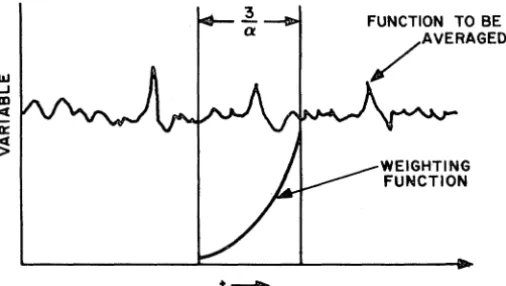
The value of the constant, ex , determines how fast past information becomes obsolete. It is chosen arbitrarily to be large enough to filter out non-essential random fluctuations and small enough not to obscure long term trends. A useful rule of thumb can be developed by examining the response of the circuit of Figure 4. If f(t) changes abruptly (step input), f(t) will follow gradually, making 95% of the change in 3 time constants or a time interval of 3/ex. In other words, as shown in Figure 5, after
1&1 ...J
III
c(
0:
~
t - +
FUNCTION TO BE /AVERAGED
Figure 5. The EMP Mean of a Continuous Variable Provides a Measure of the Averoge of the Variable for a Continuously Updated Fixed Time Interval. Note the 95% decrease in the value of the weighting function over a period of length 3/a.
This means that the weighted average at time, t, is virtually independent of values that occurred prior to time t - 3/a.
three time constants, the integrator has forgotten 95% of the information it had before the step change. Consequemly, the EMP average defined by Equation 8 is an estimate* of the mean over a time interval approximately equal to 3/ex.
*/1 a 99% criterion were used, the time interval would be approxi-mately 51a.
In the circuit of Figure 4 it is obvious that an initial condition applied to the integrator will improve the computed average at the beginning. This value should represent a good guess as to the nominal or expected mean value of f(t). One normally would have such an estimate available. If itis a good estimate, the com-puted average will be reasonable from the start; if it is a bad one, it will not make any difference after about three to five time constants.
THE VARIANCE
A second important statistical parameter is the variance which is used to give a basic measure of the distribution of a population. It is defined as the square of the standard deviation and is equal to the mean- squared deviation of the variable from its mean. For discrete data, an estimate of the variance is obtained with the summation
(11)
The term N - 1 corresponds to the number of degrees of freedom involved in the calculation of the estimates of the variance (3); practical con-siderations dictate that the number of samples, N, will be larger than one.
In a manner similiar to the definition of the mean, Otterman (2) defines the EMP variance as
.2(T)
~
{[f(t) _ I(t)]"
e -(T -t) dt
(12)-00
which, based on the preceding development of the EMP mean, will be recognized as the weighted average of the square of the deviation of the variable from its mean.
The computer circuit for calculating an estimate of the EMP variance is developed easily without re-course to mathematical manipulations. From the definition, and remembering that averaging is ac-complished by the first-order filter circuit, the following operations are required:
[image:5.617.19.274.108.191.2] [image:5.617.23.276.429.572.2]2) subtract the mean from the current value of f(t).
3) square the difference of the mean from the current value of f(t).
4) average the square with a second filter circuit.
From these requirements the circuit of Figure 6 is derived easily.
Figure 6. Analog Circuit for Calculatior of the EMP Estimate of the Variance
Example: The LD Steel Process can be used as an example of the use of the EMP mean and variance for the control of a process. This is the oxygen steel making process wherein it is possible to con-trol bath temperatures without an external fuel supply by charging the vessel with materials that are thermally balanced. The charge materials con-sist of hot metal (iron), scrap, and lime.
The hot metal temperature can range from 2200°F to 2600°F, and, hence, it is necessary to measure the temperature of the iron to obtain a correct thermal balance.
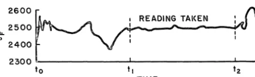
A two-color radiation pyrometer method is used to measure the iron temperature while it is being poured into the vessel. A typical trace is shown in Figure 7. (For further details of the process the reader is referred to reference 4.)
lL
o
2600
2500
2400
READING TAKEN
2300 L-______________ ~ ________________ ~~
to
Figure 7. Plot of Hot Metal Temperature vs Time for the LD Steel Process
The initial variations in temperature, t o<t<tl, are due to the presence of smoke and the forma-tion of voids in the pour. The operator disregards
these readings until the smoke has been blown away (by a fan) and smooth pouring is established. Note that even after these conditions have been attained, the temperature measurement, t 1<t<t2, is subject to fluctuations.
At present, the "temperature" reading is inserted manually into the charge balance computer (the mean value of temperature is "guesstimated" by the operator). This could be automated easily with an EMP mean value circuit since the transducer signal is a continuous electrical signal. The condi-tion that the reading of the mean value circuit should not be used at the beginning of the time history, t<tl, for reasons mentioned previously, can be automated by using the standard deviation (variance) as a control criterion, i.e., when 0'2(T)
is greater than a reference value, do not use f(T) , when 0' 2(T) is less than a reference value, use f(T). The reference value chosen will depend on the maximum variance expected during smooth pour conditions. This can be mechanized readily on the analog computer by means of a comparator.
With this simple technique a better estimate of the mean temperature could be inserted into the charge computer automatically and economically.
A UTOCORRE LA TION
The autocorrelation function, defined as an integral between fixed limits, is converted easily to a con-tinuous EMP autocorrelation function, ¢ (T), by the definition
T
• (T)
~
1
fIt) fIt -;) e -a (T - t) dt-00
(13)
Cross correlation also could be accomplished by the substitution of a second function, g(t), into the time delay box, r, shown in Figure 8, so that the output of the delay box is g(t - r) and the output of the multiplier becomes -
[f(t)]
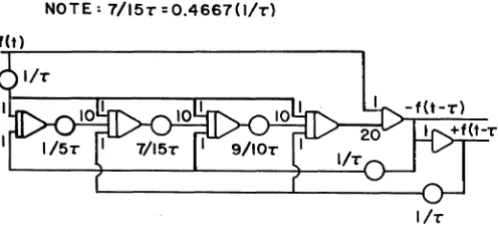
[g(t - T)] • [image:6.618.62.322.200.263.2] [image:6.618.67.316.575.650.2] [image:6.618.346.568.644.708.2]Reasonable time delays are obtained easily by as-sembling linear analog computing components. Fig-ure 9 shows a fourth-order Pade circuit for
genera-NOTE: 7/15. = O.4667( 1/.)
1/.
Figure 9. Circuit for Fourth-Order Pade Approximation for Ideal Time Delay of Magnitude r (5)
ting a time delay, T. This circuit is accurate to with-in 1 degree of phase shift for input frequencies in f(t) such that the product of the maximum useful signal frequency, wm , with the time delay, T, shall not exceed 6.5 radians, i.e.,
TW
<
6. 5 radiansm- (14)
FOURIER AND POWER SPECTRUM ANALYSIS
The EMP Fourier transform of f(t) is defined as
T
F(w) =
1
f(t) e -aCT - t) e -jwt dt (15)-00 or
-j wT F(w) = a e
(16)
f(t) e -aCT - t) ejw(T - t) dt
The EMP power spectrum is defined as
(17)
pew) = \F(w) \ 2
= .2
[100
f(t) e-·(T - t) Cos w (T _ t) dt] 2+ .2
[l
f(t) e -.(T - t) Sinw(T - t) dtr
Figure 10 shows the analog circuit for obtaining the power spectrum, pew), of the Fourier transform,
F(w). The real component, E 1, is formed from the
transfer function
E 1 · (P + a)a
f(t) - - 2 2
(P +a) + w
(18)
and the imaginary component, E2, from
aw
2 2
(P +a) + w
(19)
Note that this circuit gives pew) at one value of w. The parameter, w, can be changed merely by changing the two potentiometers labelled
"w"
pew)
Figure 10. Circuit for Calculation of EMP Fourier Transform and Power Spectrum
An alternative is to build similar circuits in parallel, all having the same input, f(t) , and dif-fering only in the setting of w. This will allow many points of the power spectrum to be obtained
simultaneously.
REGRESSION ANALYSIS
Until now, only those statistical parameters that describe a single population--mean, variance, power spectrum, etc.--have been discussed. Of interest, also, is the method of statistics whereby relationships between two or more populations, representing different variables, are found. This method is called' 'regression analysis".
There are many types of regression---linear, quadratic, high order, multivariate, etc. These terms refer to the type of expression used to re-late the variables. For example,
y=mx+b (linear regression)
2
Y
=
ax + bx + c (quadratic regression)(20)
[image:7.615.25.274.95.214.2] [image:7.615.302.549.283.394.2] [image:7.615.23.269.588.711.2]Regression consists, essentially, of finding the best "fit" to a set of data using a least-squares criterion. While several authors have hinted at obtaining a "least squares" fit by analog techniques for special cases, none have shown a straight-forward solution to the regression problem as de-fined above for continuous variables.
As an illustration of how least squares fitting would be performed on the analog computer,
con-sider the linear case defined by Equation 20. For this general equation it can be shown (6) that the following two equations will define the unknown parameters m and b, the slope and intercept of the line, respectively.
N
"'"" X.Y.
L..J
1 1i=l
N
m
2:
Xi + Nbi=l
N
+ L X i
i=l
(22)
(23)
Since X and Y will be continuous functions of time, the discrete summation from 1 to N can be replaced by a time integral where the total time, t, is proportional to N. Therefore, Equa-tions 22 and 23 become
f
t XY dto
t
mf.
Xdt+bt ot
d t + b i Xdt
(24)
(25)
These two equations can be solved simultaneously to yield m and b as follows:
t t
b
=!a
Y dt - mfax
dt(26)
t
(27)
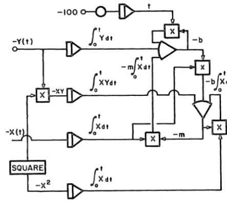
Figure 11 shows the analog computer circuit for calculating the "least squares" parameters m
and b using the definite integral. One should note
-V(t)
,
i
XVdtFigure 11. Circuit for Obtaining the "Least Squares" Regression Parameters!!! and ~
that in calculating m and b from the definite in-tegral we form an "algebraic" loop. This brings up the question of circuit stability. It can be shown" that once the computation is under way, (t>O), the loop will be stable unless X is constant. However, if X is constant it cannot be used as an independent variable in a correlation study. Overloads at the very beginning of the computation (a region of no interest) can be taken care of with feedback limiters on the division amplifiers, or by using a "steepest descent" division circuit (7).
It should be observed that m and b are defined at every instant of time. For small values of t (corresponding to small sample size), the estimates of m and b will be relatively insignificant and, hence, will be changing rapidly. As the time in-terval increases, however, the values of m and b
become more significant and actually should reach "steady state" or non-changing values.
The technique for linear regression can be extended to quadratic or higher order regressions, it then being necessary to define a new set of equations--such as Equations 22 and 23-- for determining the unknown parameters of the regression system. Once the equations are defined, they can be con-verted to continuous integrals and instrumented by standard analog techniques.
Again we are dealing with continuous signals, which means that there must be a limit of the integration interval if circuits such as that of Figure 11 are to
[image:8.618.346.568.88.284.2] [image:8.618.78.313.448.558.2]be used. Just as before, the need for resetting of integrators can be eliminated by converting the equations for m and b to EMP equations and, theby, obtaining truly continuous estimates of the re-gression parameters.
Equations 22 and 23 are rewritten by dividing through N. This yields
N N
L
Yi L X ii=l i=l
+ b m
N
N (28)
N N N
L
X.Y.LX~
L X i
1 1
i=l i=l
+ b i=l
N m N N (29)
Recalling the correspondence between EMP vari-ables and discrete summations, one can transform Equations 28 and 29 immediately into continuous EMP notation which gives
mX + b (30)
(31)
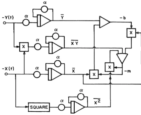
where m and b are now the EMP estimates of the regression parameters. The analog circuit required is shown in Figure 12. The statements made with regard to the stability of the circuit shown in Fig-ure 11 apply also to the algebraic loop found in the Figure 12 circuit,
It should be observed that time has, in effect, been taken out of the problem by the conversion to EMP variables. There is no longer any need to "reset" the integrators since they are now serving as con-volution circuits rather than pure accumulators. It
follows that circuits similiar to those shown can be instrumented for continuous higher order and con-tinuous multi-variable regressions. All that is reo quired is more analog computing equipment.
Figure 12. Unsealed Analog Circuit for Calculation of Continuous EMP Values of Regression
Parameters I:!! and ~
CONCLUSIONS
The conversion of statistical parameters to EMP variables enables data analysis to be performed continuously through the use of relatively simple analog circuits. Limits on the size of the integra-tion interval normally encountered with continuous signals have been eliminated; the need to "reset" the integrators is no longer required since they are now serving as convolution circuits rather than pure accumulators. A continuous estimate of statistical parameters can be calculated readily.
[image:9.615.296.543.41.243.2]APPENDIX I: REFERENCES
(1) Davenport, W.B., Jr., and W.L. Root: "An Introduction to the Theory of Random Signals and Noise", McGraw-Hill Book Company, Inc., New York, 1958.
(2) Otterman, Joseph: "The Properties and Methods for Computation of Exponentially Mapped Past Statistical Variables", IRE TRANS. on Automatic Control, Volume AC-5 Number 1, January 1960, pp. 11-17.
(3) Volk, William: "Applied Statistics for Engineers", McGraw-Hill Book Company, Inc., New York, 1958, p. 136.
(4) Slatosky, W.J.: "End Point Temperature Control in LD Steel Making", Journal of Metals, Volume 12, March 1960, pp. 226-230.
(5) Brenner, M.M., and J.D. Kennedy: "Dead Time Simulation for Electronic Analog Com-puters", National Simulation Council, December 11, 1957.
(6) Widder, D.V.: Advanced Calculus, Prentice-Hall, 1947, P. 108.
(7) Favreau, R.R.: "Dividing Circuit Obtained by Applying Method of Steepest Ascent", Princeton Computation Center Report 132, Electronic Associates, Inc., Prmceton, New Jersey.
EAr
ELECTRONIC ASSOCIATES, INC. Long Branch, New JerseyADVANCED SYSTEMS ANALYSIS AND COMPUTATION SERVICES/ANALOG COMPUTERS/HYBRID ANALOG·DIGITAL COMPUTATION EQUIPMENT/SIMULATION SYSTEMS/
SCIENTIFIC AND LABORATORY INSTRUMENTS/INDUSTRIAL PROCESS CONTROL SYSTEMS/PHOTOGRAMMETRIC EQUIPMENT/RANGE INSTRUMENTATION SYSTEMS/TEST