Customer Success Using Deep Learning

(1)

Customer

Success

U

sing

Deep

Learning

Shobha

Deepthi

V

1,∗

,

Sumith

Reddi

Baddam

2

,

Vignesh

Thangaraju

2

1_Member_of_Technical_Staff,_Cisco_Systems_India_Pvt._Ltd.

2_Engineer,_Cisco_Systems_India_Pvt._Ltd.

Abstract

Customer Success is gaining priority for Organi-zations in transforming to recurring revenue business model. For this we need to shift our paradigm from being a “reactive troubleshooting” to “proactively advising” our customers. As part of this transformation various capabilities are being built, to capture customer data, have smart agents that collect infor-mation from customer networks to predict a failure before it happens and to advise the customer of the resolution. Products can be both hardware and software. It is trickier to predict a failure or an issue beforehand in software when compared to hardware because in hardware there are predefined set of symptoms for a failure. In software, predicting an issue beforehand means knowing and understanding what code is going in with each commit, defect or an enhancement. In most cases, defects found during internal testing, which are often neglected, crop up as customer issues at a later point in time. In this paper, we propose a solution to predict the potential defects that the customer might find after the release of the product using LSTM and CNN. We also predict the time (weeks or months) within which the customer might face this issue. This knowledge helps the teams to prioritize the defects and proactively resolve them on time before going live with known backlog of issues. Thus improving the quality of product that we deliver. Post production this can help proactively advise customers on these known issues that he might face and recommend a software patch or upgrade path. This paper is aimed at reducing internal failures cost component of Cost of Quality leads to Customer Retention and Success.

Keywords

Customer Success, Deep Learning

1 Introduction

Cost of quality is a methodology that allows an organization to determine the extent to which its resources are used for activities that prevent poor quality, that appraise the quality of the organization’s products or services, and that result from internal and external failures. Having such information

allows an organization to determine the potential savings to be gained by implementing process improvements. There are four categories: internal failure costs (costs associated with defects found before the customer receives the product or service), external failure costs (costs associated with defects found after the customer receives the product or service), appraisal costs (costs incurred to determine the degree of conformance to quality requirements) and prevention costs (costs incurred to keep failure and appraisal costs to a minimum).

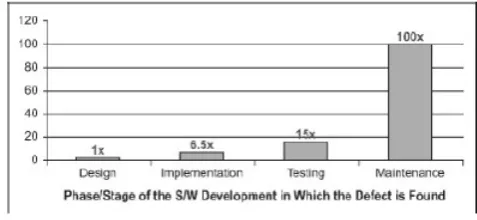
[image:1.595.307.546.557.667.2]

In Software Development Life Cycle, most of the issues identified, starting from unit testing till beta testing, are either marked unreproducible or deprioritized, because of two reasons, either there is not enough data, or not enough analysis is done to reproduce the issue. Any issue identified earlier during development stage, is easier and cheaper to fix and also the early detection and prioritization of the defects ensures a product with good quality to end customers. There have been studies which state the cost of fixing a defect as it moves through the later stages of development life cycle grows exponentially[1].

Figure 1. Phase/stage of software development in which defect is found

(2)

[image:2.595.44.292.156.653.2]

release was four to five times as much as one uncovered during the design, and up to 100 times more than one identified in the maintenance phase[1].

Table 1. Bug report attributes, N-categorical, C-continuous, T-text

Attribute (Type) Short Description

Component (N) Group or list of files with a targeted funtioncality. This represents a feature or set of features.eg.aaa

Product (N) Product in which the defect or issue is reported. This will also capture platform eg. asr9k Severity (C) Severity of the issue report. Takes

a value between 1-6. 1 being the most sever issue

Assigner (N) Engineer who is assigned to work on this issue

Month opened (C) Month in which the issue was reported

Year opened (C) Year in which the issue was reported

Submitter (N) Engineer who reported the issue Status (N) Status of the issue reported. Eg.

Open, Closed, Duplicate, Unreproducible

Headline (T) Short Description of the issues Description (T) Detailed explanation of the issue,

failure logs, code chunks etc. Found (N) Phase during which the issue was

found. Eg, development, sys-test, customer-use

Priority (N) Development prirority for the bug Category (N) Defect category. Eg. Infra,

performance

Attribute (T) Tags or key words associated Submitted-on (C) Day the defect was submitted IFD_CFD_Date (C) Day the internaly found defect

was also reported by customer or the day this defect is marked as duplicate of customer reported issue

IFD_CFD_INDIC (N) This indicates whether the bug became a potential customer issue or not (1 or 0)

Apart from identifying an issue, it is equally important to analyze, prioritize and fix these issues. Focus for our problem is to help engineers with a recommended analysis on potential issues that will be reported by the customers. We also provide a solution to estimate the time it takes to to fix these issues even before customer might report it.

For this, we look at historical data of defects/issues reported during development stage and the issues which were reported by the customer. In this data we consider various defect

attri-butes and unstructured data like the defect description, failure logs etc., to extract the intent and sensitivity of the issue. This is an ensemble model to predict a potential customer issue and lead time before which it needs to be fixed.

2 Data Analysis

As it can be seen, the problem is two-fold. First is to predict which internally found defect could be a potential customer issue. Secondly, to predict how many weeks or months after a release would the customer face the issue and report the same.

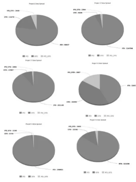
Figure 2. Data spreadIFD - internally found defect, CFD - customer found defect, IFD_CFD - issue that was found internally was also found by customer

We collected historical data for 3 years for different Cisco product families. This defect data has both internally found issues, issues found during testing phases and customer found issues, issues which customer has reported after using the software. If the same internally found issue is reported by customer as well, one of them would be reported as duplicate. “Found” attribute in defect data will differentiate a customer reported issue from internal found issue.

Data comprises of

• Continuous features

• Categorical features

[image:2.595.309.541.244.555.2]

(3)

Continuous data here represents the date when the issue was re-ported, the date when it got converted to a customer issue, age of the defect, number of service request cases attached with it, etc. Categorical variables define complexity, nature and im-pact of the issue reported. Text data has a detailed description, analysis and resolution of the issue.

The table [1] lists the fields in the dataset. Those marked with (C) are continuous, (N) are categorical or numeric data and (T) are text/ unstructured data. Continuous data helps in identifying the significance of time for an event in this a custo-mer reported issue. The last two variables IFD_CFD_Date and IFD_CFD_INDIC are computed fields. Looking at a defects life cycle, date when a internally found defect is converted as customer found defect is calculated. IFD_CFD_INDIC is our target variable that classifies a defect as a potential Customer issue or not.

2,069,035 defects over a period of 3 years is considered for this problem. Among these defects 148,188 were customer issues and 17,759 were potential customer defects i.e, the de-fects that were internally found but later reported as customer issues as well. Below is the spread across multiple projects, it can be seen that the % of potential customer data is less which causes imbalance in data for classification. This is one of the challenges with data and how it is handled is discussed in later sections of this paper.

For the first use case, which is to classify a defect as potential customer issue, two models are built,

• LSTM, a variant of Recurrent Neural Network

• XGBoost

The LSTM (Long Short-term memory) model is built for the textual descriptions of the bugs in Keras. First defects are sampled by project, to pre-process the text data by lemmati-zing and tokenilemmati-zing it and train the model. Before training the LSTM words are embedded into vectors of same dimensions. The categorical and continuous attributes in the dataset are fed to XGboost model for training. Both these models output the confidence or probability which we concoct using an ensemble method and arrive at the final prediction of the propensity that the bug will be reported by the customer.

The second use-case is to predict the time it takes for a custo-mer to find and report the bug from its day of release. For this Deep Neural Network regression model is used. This model considers the continuous and categorical attributes mentioned above and predicts the timeframe. Before training, attributes of the defect are processed and converted into tensors for feature extraction.

3 Prediction of Customer Found

De-fects

Prediction of internally found defects that have the pro-pensity to become a customer found defect is classification problem whether a customer will face the issue or not.

Major difficulties about this problem are the imbalances in the dataset, variety of features (eg. text, continuous and categorical) and dealing with missing values.

Our solution includes two models to be built, one for the tex-tual description data and the other for continuous and categori-cal features for each bug. Both these models output the proba-bilities of the bug becoming a potential customer issue and we then use feature-weighted linear stacking ensemble technique to make the final prediction.

3.1 Text classification using CNN and LSTM

Major difficulty with textual descriptions is that they vary a lot in length, have lots of references to product names, symbols and abbreviations, email addresses and sometimes they are not proper english sentences. Our solution deals with handling such cases and building a convolutional neural network on top of LSTM recurrent neural networks model.

The dataset contains 2,069,035 defects over a period of 3 years. Among these bugs 148,188 bugs are customer issues (these include both customer-only found issues and internally found issue that were also reported by customer). We split this data into 70% training set and 30% validation set.

The data is loaded into Keras framework and preprocessed. As a first step we build the vocabulary of words and also the frequency matrix. The words are then replaced by integers that indicate the ordered frequency of integers. Only top 10,000 words are considered. Now the text descriptions are a sequence of integers.

We use a technique called word embedding where words are encoded as real valued vectors in high dimensional space and the similarity between words in terms of meaning translates to closeness in the vector space. We map each word in the vocabulary into a fixed length (64) real valued vector and the other words which are not in the top 10,000 are replaced with zeros. Also to deal with varying description length we constrain each description to be 300 words, truncating long descriptions and padding the shorter ones.

(4)

features and filter lengths of 5 and a max pool layer of length 2. The next layer is the LSTM layer with 100 memory units. Since our task is to predict if a bug gets converted or not, we use a dense output layer with single neuron and a sigmoid activation function to make 0 or 1 predictions for the two classes. Dropout layer is also added between CNN and LSTM layers and LSTM and Dense output layers to avoid overfitting the problem.

We use a log loss function because it is a binary classifica-tion along with ADAM optimizaclassifica-tion algorithm. The model is run for just 100 epochs so that it won’t over-fit the problem. The output for each defect/bug will be a probability of the bug becoming a potential customer issue.

3.2 XGBoost for classification

XGBoost is an advanced implementation of gradient boos-ting algorithm[3]. We build this model using the continuous and categorical features in our dataset. The major challenge for building this model is the imbalance in the dataset. Bugs which are internally found rarely get converted to customer issue, that is only 1-18% bugs get converted2. This imbalance effects the algorithm to not give accurate results.

To deal with this we worked on random under-sampling of the majority class, random over-sampling of the minority class and cluster based over-sampling. But all these methods failed resulting the model to over-fit and under-perform, because in case of under-sampling we were missing on important data points and in case of over sampling we merely duplicated the data points from the minority class.

We then adapted an algorithm called Synthetic Minority Over-Sampling Technique (SMOTE), which is an informed over-sampling method[4]. We followed this technique to avoid the problem of overfitting which occurred when the exact replicas or duplicates of minority class were added to the da-taset. In this algorithm a subset of minority class is taken and new synthetic similar instances were created. These synthetic instances are then added to the dataset. The advantage of this technique is that there is no loss of information and no duplicates as well.

SMOTE works by calculating the distance between the majority class datapoints and minority class data points. The continuous features can easily be synthetically generated but for categorical variables in order to be able to calculate such distances we need to vectorize them first. We convert the categorical features into one hot vectors and generate the synthetic data points.

Imputing the missing values with XGBoost algorithm is easy. We transform the features with missing values into matrix and then XGBoost captures the trends in missing values and handle them internally. Before training the model, we first run a feature importance plot (see 3, 4) to know the useful

features. We tune the parameters using a grid search on a set of parameter values by evaluating them against the validation set.

For validation of the model we used a 5-fold-cross validation[5]. The data is broken into 5 sets of equal size. The model is trained using 4 datasets and tested with the remaining dataset. The process is repeated 5 times with each of 5 datasets as validation set. The results of the 5 folds then are averaged to evaluate the performance of the model. This process is run for different parameter sets and the most optimal one is selected.

Confusion matrix (see 5) is plotted on the validation set. Af-ter the training and validation, we predict the outputs for the testing dataset. The output is a probability of that bug beco-ming a customer found defect.

3.3 Evaluation

Ensemble method is designed to boost predictive accuracy by blending the predictions of these two machine learning models. The output probabilities from both our models above are combined to make a final prediction. For this we use XGBoost model[6]. This model finds the patterns in the output probabilities and makes final prediction. The parameter tuning for this is determined using the meta-data and the grid search.

We use precision (P), recall (R) and the area under the re-ceiver operating characteristic curve (AUC) statistic for me-asuring the performance of the prediction models. Precision denotes the proportion of correctly predicted customer found defects, P = TP/(TP + FP). Recall represents the proportion of true positives of all customer found defects, R = TP/(TP + FN). AUC can be interpreted as the probability, that, when randomly selecting a positive and negative example the model assigns a higher score to positive example[7]. In our case the positive example is a bug which is customer found defect.

4 Prediction of time to find a bug

Prediction of time (weeks or months) taken by a customer to find an internally found bug is a regression problem where we use categorical and continuous features like the priority of the bug, status, component it belongs to, project it is from, month and year it was created, the assigner and submitter of the bug. Our prediction variable here is the number of days between the date it was found by the internal testing team and the date customer has reported it. A deep neural networks regressor model is built in TensorFlow framework[8].

4.1 Feature selection and preprocessing

(5)

continuous and target feature names in different variables. When building a model in TensorFlow the input data needs to be specified by an Input Builder function which constructs the input data in the form of Tensors. The continuous features are stored in constant tensors whereas the categorical features are stored in sparse tensors. Once the input for TensorFlow graph has been constructed we do feature selection and feature engineering for the model.

4.2 Deep Neural Network Architecture

The 3-layer deep neural network regressor model is built and trained in TensorFlow to predict the number of days it takes a customer to report a bug that was internally found during testing. Building a model in TensorFlow is nothing but building a computational graph which can be any mathemati-cal operation that the TensorFlow supports[9].

Our model has an input layer of fixed size, 3 hidden layers with 64, 32 and 10 neurons respectively and a single output neuron which outputs a continuous value. We define mean sum of squared error as our loss function and set the opti-mizer, that is, back propagation algorithm as ADAM optimizer. Once the graph is built, we initialize the weights and bia-ses to compile the variables. To train the model, we create a session and run the graph in that session. The training data is first divided into batches so that it can be ingested. The ba-tches are first preprocessed, augmented and then fed into the deep neural network for training. The model then gets trained incrementally. The execution happens for 1000 epochs. The model is validated against the validation set. After performing the training, the model is stored in a directory so that it can be later used for prediction on testing data.

5 Results

The model is tested acroos 11 projects over 1 million bugs, The results for a single project accross the three different mo-dels is shown below.

The relationship and importance of the above features were considered for the prediction of a defect becoming a potential customer issue and for the time it takes for a customer to find and report this issue from the day of release.

[image:5.595.335.515.144.325.2]

5.1 Classification of customer issue using

XG-Boost

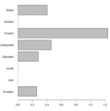
Figure 3 intuitively explains what features will be useful for classifying a bug becoming potential customer issue. So in our XGBoost model, we considered component, status, product, assigner and submitter features.

A grid search run has been performed on the model to tune the parameters for a high accuracy and precision.

Figure 3. Importance plot for classification of customer issue

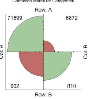
[image:5.595.344.513.486.678.2]

(6)

[image:6.595.343.514.89.279.2]

Figure 5. Confusion matrix for XGBoost model

The figure 5 represents a confusion matrix for test set, where True is the actual class that bug belongs to and Pred is the model prediction.

We use sensitivity, specificity and accuracy metrics to evalu-ate the model. The precision of the model correctly predicting a customer issue is

Specificity = _{T N}T N₊_{F P} = 0.912

Sensitivity/Recall = _{T P}T P₊_{F N} = 0.573

Accuracy=_{T P}₊_{T N}T P+₊T N_{F N}₊_{F P} = 0.905

That is, the model is 90.5% accurate while predicting if a bug is a customer issue or not and the true positive rate for predicting a customer issue is 0.573.

5.2 Classification of customer issue using CNN

and LSTM

The texual descriptions of the defects/bugs are used for the classification of potential customer issue. The words in the descriptions are converted into word embeddings and passed to a convolutional neural networks where the network picks the invariant features and passes them to an LSTM layer. The final output is the probability of a bug becoming a potencial customer issue.

Figure 6, shows the confusion matrix of this CNN-LSTM model for the validation set,

Sensitivity, Specificity and Accuracy are calculated as the metrics of accuracy of the model. The model’s sensitivity is 0.709, specificity is 0.932 and accuracy is 0.925. The results show that the model is highly precise while predicting a custo-mer issue and the overall accuracy of the model is,

[image:6.595.84.252.97.286.2]

Specificity=_{T N}T N₊_{F P} =0.932

Figure 6. Confusion matrix for CNN - LSTM model

Sensitivity/Recall =_{T P}T P₊_{F N} =0.709 Accuracy = _{T P}₊_{T N}T P+₊T N_{F P}₊_{F N}= 92.5%

That is, the model is 73.1% accurate while predicting if a bug is a customer issue or not and the true positive rate for predicting a customer issue is 0.709.

5.3 Ensemble predictions

[image:6.595.342.512.554.744.2]

Extreme gradient boosting model is used to make the final prediction regarding the propensity of a bug becoming a custo-mer issue. This model runs by blending the predictions of the two models.

Figure below, shows the confusion matrix of this XGBoost ensemble model for the validation set,

(7)

Precision, recall and F-score are calculated as the metrics of accuracy of the model. The model’s specificity is 0.969, recall is 0.967. The results show that the model is highly precise while predicting a customer issue and the overall accuracy of the model is,

Specificity= _{T N}T N₊_{F P} = 0.969

Sensitivity/Recall = _{T P}T P₊_{F N} = 0.967

Accuracy =_{T P}₊_{T N}T P+₊T N_{F P}₊_{F N}= 97.54%

That is, the model is 97.54% accurate while predicting if a bug will become a customer issue or not and the true positive rate for predicting a customer issue is 0.967.

We see that out of 1412 customer issues in total, we pre-dicted 1365 accurately and 47 were misclassified and in the case of predicting a non-customer issue the model was correct for 76075 bugs and wrong for 2396 bugs.

[image:7.595.93.244.156.215.2]

5.4 Prediction of time to be taken by a customer

to find the issue using Deep Neural Network

Figure 4, shows that the useful features for the prediction of the number days are, month in which the release was made, product in which the issue was found, severity of the defect/bug, status of the defect, and component it belongs to. So we consider all these features for the model prediction.

The 3-layer Deep Neural network regressor model is built and trained to predict the number of days it takes a customer to find an issue from the date of release. The data set has 1033 customer issues.

The loss function is defined as the Mean Sum of Squared Error. ADAM optimizer is uesd for the backpropagation algo-rithm. The model is run for 1000 epochs and the loss for the final step is 33.1126 for the training dataset. The validation dataset has a loss of 831.94. The mean difference in the pre-dicted number of days and the actual number of days it took was around 20 days. So whenever the model makes a pre-diction of the number of days we consider a variance 20 days.

6 Conclusion and Future work

The models were run for different set of products and platforms and classification had 97.5% accuracy and were able to predict the time frame that the issue would be uncovered by customer with a variance of 20 days. The model training is run on monthly basis and it is tested weekly on all the new bugs that are filed in that particular week.

This approach can be taken with any products that follow the typical development life cycle and defect management system. A standard quality management system captures the details of the issue in the same format of summary, description, severity, logs, failure notes etc. Before the go-live the model

can be run on the all internally found defects to identify which could possibly impact the cost of quality post production.

Post production, most of the time is spent in figuring if it is a known issue by scanning through a sea of internal failures de-fects. This projected list of probable customer issues will have a targeted list to work with for the Customer Facing team, in quickly apprising the customer of the issue and possible reso-lution time.

REFERENCES

[1] M. Soni, "Defect prevention: Reducing costs and enhancing quality," iSixSigma. com, vol. 19, 2006.

[2] J. Wang, L.-C. Yu, K. R. Lai, and X. Zhang, "Dimensional sen-timent analysis using a regional cnn-lstm model," in ACL 2016 Proceedings of the 54th Annual Meeting of the Association for Computational Linguistics. Berlin, Germany, vol. 2, 2016, pp. 225-230.

[3] T. Chen and C. Guestrin, "Xgboost: A scalable tree boosting system," in Proceedings of the 22nd acm sigkdd international conference on knowledge discovery and data mining. ACM, 2016, pp. 785-794.

[4] C. Bunkhumpornpat, K. Sinapiromsaran, and C. Lursinsap, Safe-Level- SMOTE: Safe-Level-Synthetic Minority Over-Sampling TEchnique for Handling the Class Imbalanced Problem. Springer Berlin Heidelberg, 2009, pp. 475-482.

[5] R. Kohavi et al., "A study of cross-validation and bootstrap for accuracy estimation and model selection," in Ijcai, vol. 14, no. 2. Stanford, CA, 1995, pp. 1137-1145.

[6] J. Sill, G. TakÃ¡cs, L. Mackey, and D. Lin, "Feature-weighted linear stacking," arXiv preprint arXiv:0911.0460, 2009.

[7] J. A. Hanley and B. J. McNeil, "The meaning and use of the area under a receiver operating characteristic (roc) curve." Radiology, vol. 143, no. 1, pp. 29-36, 1982.

[8] M. Abadi, A. Agarwal, P. Barham, E. Brevdo, Z. Chen, C. Citro, G. S. Corrado, A. Davis, J. Dean, M. Devin et al., "Tensorflow: Large-scale machine learning on heterogeneous distributed systems," arXiv preprint arXiv:1603.04467, 2016.