COST SENSITIVE META LEARNING
SAMAR ALI SHILBAYEH
SCHOOL OF COMPUTING, SCIENCE AND ENGINEERING
UNIVERSITY OF SALFORD
MANCHESTER, UK
i
Contents
ACKNOWLEDGMENTS vi
ABSTRACT vii
CHAPTER ONE: INTRODUCTION 1
1.1 Research Aim, Objectives and Motivation 1
1.2 Research Motivation 1
1.3 Research Objectives 2
1.4 Research Methodology 2
1.5 Outline of Thesis 6
CHAPTER TWO: BACKGROUND AND LITERATURE REVIEW 7
2.1 Cost-Sensitive Learning 7
2.1.1 Cost-Sensitive Background 7
2.1.2 Cost-Sensitive Learning in the Imbalanced Data Problem 8
2.2 Meta-Learning Background and Literature Review 15
2.2.1 Meta-Learning Perspective and Overview 16
2.2.2 Meta-Learning Goals and Benefits 17
2.2.3 Meta-Learning Literature Review 18
2.3 Feature Selection 21
2.3.1 Feature Selection Background 21
2.3.2 Feature Selection Literature Review 26
2.3.3 Feature Selection in Meta-learning Work 27
2.4 Active Learning 28
2.4.1 Active Learning Background 29
2.4.2 Active Learning in Meta-learning Scenarios 34
2.4.3 Active Learning Literature Review 36
2.5 Summary of the Literature Review 39
CHAPTER THREE: COST SENSITIVE META LEARNING 45
3.1 Cost-Sensitive Meta-learning 45
ii
3.1.2 Base Learning Process 57
3.1.3 Performance Evaluation 60
3.1.4 Meta-Learning Process 60
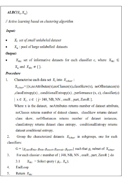
3.2 Development of Active Learning Based on Clustering 62
3.3 Summary of Cost-Sensitive Meta-Learning Work and Active Learning 77 CHAPTER FOUR: EMPRICAL EVALUATION OF NEW COST SENSTIVE
META-LEARNING SYSTEM 78
4.1 Feature Selection Experiment 78
4.1.1 Evaluating Feature Selection Approaches 79
4.1.2 Developing Meta-Knowledge for Feature Selection 86
4.2 Cost-Sensitive Learning Experiment 96
4.2.1 Cost-Sensitive Experiment Methodology 97
4.2.2 Cost-Sensitive Meta-Learning System Evaluation 109
4.2.3 Conclusion 125
4.3 Active Learning 127
4.3.1 ALBC Comparison Result with Random Selection 129
4.3.2 Results Discussion 133
4.3.3 Clustering Based on Best Cluster 133
4.3.4 Conclusion 134
CHAPTER FIVE: CONCLUSION AND FUTURE WORK 136
5.1 A Review of the Research Objectives 137
5.2 Future Work 141
Appendix A Cost-Sensitive Meta-knowledge Decision Trees 150
A1. Feature Selection Meta-knowledge Decision Tree 150
A2. Cost-Sensitive Meta-knowledge Decision Trees 154
Appendix B Meta-Learning Cost-Senstive and Active Learning design 162
B1.Cost- Sensitive Meta-knowledge System Design 162
Feature Selection Meta-Knowledge Development 162
Cost sensitive Meta-Knowledge Development 169
B2.Active Learning Based on Clustering 183
iii
List of figures
Figure 2-1: Wrapper and Filter methods ... 25
Figure 2-2: Uncertainty samples that are outliers ... 33
Figure 2-3: Datasetoid generation ... 38
Figure 3-1:Meta-Learning for cost sensitive learning ... 47
Figure 3-2: Feature selection meta-knowledge development ... 50
Figure 3-3: Cost sensitive meta-knowledge development ... 51
Figure 3-4: Information theoretic measures on different datasets ... 57
Figure 3-5: Examples of strong and weak clusters ... 65
Figure 3-6: Active learning based on clustering ... 67
Figure 3-7: Illustration of classifiers specific clusters for J48 and naïve Bayes ... 68
Figure 3-8: Illustration of two clusters and their characteristics, both for J48 and naïve Bayes ... 69
Figure 3-9: The top level of the active learning algorithm ... 70
Figure 3-10: The query formulation steps ... 72
Figure 3-11: Dataset determination steps ... 73
Figure 3-12: Dataset search steps ... 74
Figure 3-13: Error Rate versus number of labelled data using ALBC ... 75
Figure 3-14: Best cluster method ... 76
Figure 4-1: Changes in classifiers accuracy after using WrapperSubSetEval with Greedy Search ... 84
Figure 4-2: Changes in classifier accuracy after using GainRatioEval with Ranker ... 84
Figure 4-3: Changes in classifier accuracy after using CfcSubEval with bestFirst ... 85
Figure 4-4: Sample of dataset characterises used to build meta-knowledge with classifier performane ... 88
Figure 4-5 : Decision tree for feature selection with accuracy (Left) ... 89
Figure 4-6: Decision tree for feature selection with accuracy (right) ... 90
Figure 4-7: Decision Tree for feature selection with misclassification cost (left) ... 93
Figure 4-8: Decision Tree for feature selection with misclassification cost (right) ... 94
Figure 4-9: Decision tree for cost-sensitive methods accuracy (right) ... 100
Figure 4-10: Decision tree for cost-sensitive methods accuracy (left) ... 101
Figure 4-11: Cost ratio with classifier accuracy ... 104
Figure 4-12: Decision tree for cost-sensitive methods in predicting cost (left) ... 106
Figure 4-13: Decision tree for cost-sensitive methods in predicting cost (right) ... 107
Figure 4-14: Cost ratio with misclassification cost ... 108
Figure 4-15: Accuracy-prediction error in diabetes dataset ... 112
Figure 4-16: Cost-prediction error in diabetes dataset ... 112
Figure 4-17: Accuracy-prediction error in credit-g dataset ... 114
Figure 4-18: Cost-prediction error in credit-g dataset ... 114
Figure 4-19: Accuracy-prediction error in Glass dataset ... 116
Figure 4-20: Cost-prediction error in Glass dataset ... 116
Figure 4-21: Accuracy-prediction error in transfusion dataset ... 118
iv
Figure 4-23: Accuracy-prediction error in heart dataset ... 120
Figure 4-24: Cost-prediction error in heart dataset ... 121
Figure 4-25: Accuracy-prediction error in vehicle dataset ... 122
Figure 4-26: Cost-prediction error in vehicle dataset ... 123
Figure 4-27: Accuracy-prediction error in vote dataset ... 124
Figure 4-28: Cost-prediction error in vote dataset ... 125
Figure 4-29: Accuracy prediction error with number of labelled examples ... 131
Figure 4-30: Accuracy prediction-error with number of labelled examples ... 132
v
List of Tables
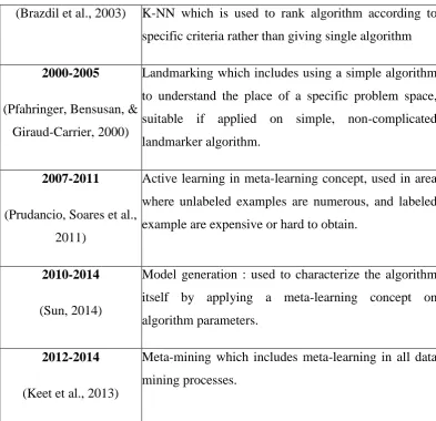
Table 2-1: Meta-learning approaches ... 40
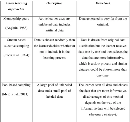
Table 2-2: Active learning approaches ... 42
Table 2-3: Active learning query strategy approaches ... 43
Table 4-1: Changes in classifiers performance accuracy using WrapperSubSetEval with Greedy Search ... 81
Table 4-2: Changes in classifier performance accuracy after using GainRatioEval with Ranker ... 82
Table 4-3: Changes in classifier performance accuracy after using CfcSubEval with bestFirst ... 83
Table 4-4:Combination of feature selection approaches, search strategies, and evaluators ... 87
Table 4-5: Misclassification cost comparison between left and right branch of feature selection tree ... 95
Table 4-6: Dataset characters for contact-lenses dataset ... 97
Table 4-7: Cost ratios ... 97
Table 4-8: Cost-sensitive approaches ... 97
Table 4-9: Accuracy categories ... 98
Table 4-10: Cost Categories ... 98
Table 4-11: Accuracy of cost-sensitive approaches with different dataset characteristics for contact-lenses 98 Table 4-12: Cost of cost-sensitive approaches with different dataset characters for contact-lenses dataset 99 Table 4-13: Different dataset accuracy using different cost-sensitive classifiers ... 102
Table 4-14: Comparison between J48 and MJ48 accuracy between balance and imbalanced dataset ... 103
Table 4-15: Accuracy and cost-prediction error in diabetes dataset ... 111
Table 4-16: Cost matrix for Credit-g dataset ... 113
Table 4-17: Accuracy and cost-prediction error in credit-g dataset ... 113
Table 4-18: Accuracy and cost-prediction error in Glass dataset ... 115
Table 4-19: Accuracy and cost-prediction error in Transfusion dataset ... 118
Table 4-20: Heart cost matrix ... 119
Table 4-21: Accuracy and cost-prediction error in heart dataset ... 120
Table 4-22: Accuracy and cost-prediction error in vehicle dataset ... 122
Table 4-23: Accuracy and cost-prediction error in vote dataset ... 124
Table 4-24: Average accuracy-prediction error for all methods used in all compared datasets ... 126
Table 4-25: Dataset characterisation for small pool of dataset ... 128
Table 4-26: Accuracy of applying different classifiers to the previous datasets with its meta-features ... 128
vi
ACKNOWLEDGMENTS
I would like to thank Allah Almighty, for giving me the strength to carry on this work and for blessing me with many generous people who have been my greatest support in both my personal and professional life. I would like to take this opportunity to express my deepest regards and gratitude to my supervisor Prof. Sunil Vadera for his dedication and support throughout this project.
Special thanks to my dad Ali and my mum Fatimah, and my sisters, Linda, Samah, Nour, Layal and Farah for all their support and assistance, without their love, help, and encouragement this journey would not have been possible.
Parts of the current PhD research have resulted in the following conferences and presentations.
Shilbayeh, S.,& Vadera,S.(2014). Feature selection in meta-learning framework. Science and Information Conference (SAI), 269-275.
Shilbayeh, S., & Vadera, S.(2013). Meta-Learning framework based on landmarking
IMSIO2013 international Conference. Proceedings of the 5th European Conference in
Intelligent Management Systems in Operations, 97-105.
Shilbayeh,S.&Vadera,S.(2012). Cost sensitive meta-learning framework. SPARC Conference. University of Salford, UK.
vii
ABSTRACT
Classification is one of the primary tasks of data mining and aims to assign a class label to unseen examples by using a model learned from a training dataset. Most of the accepted classifiers are designed to minimize the error rate but in practice data mining involves costs such as the cost of getting the data, and cost of making an error. Hence the following question arises:
Among all the available classification algorithms, and in considering a specific type of data
and cost, which is the best algorithm for my problem?
It is well known to the machine learning community that there is no single algorithm that performs best for all domains. This observation motivates the need to develop an ―algorithm selector‖ which is the work of automating the process of choosing between different algorithms given a specific domain of application.
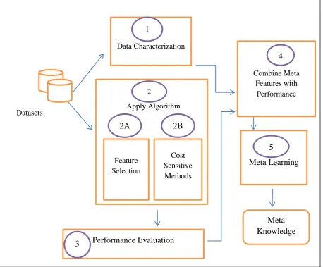
Thus, this research develops a new meta-learning system for recommending cost-sensitive classification methods. The system is based on the idea of applying machine learning to discover knowledge about the performance of different data mining algorithms. It includes components that repeatedly apply different classification methods on data sets and measuring their performance. The characteristics of the data sets, combined with the algorithm and the performance provide the training examples. A decision tree algorithm is applied on the training examples to induce the knowledge which can then be applied to recommend algorithms for new data sets, and then active learning is used to automate the ability to choose the most informative data set that should enter the learning process.
viii Although, meta-learning is not new, the task of accelerating the learning process remains an open problem, and the thesis develops a novel active learning strategy based on clustering that gives the learner the ability to choose which data to learn from and accordingly, speed up the meta-learning process.
1
1
CHAPTER ONE: INTRODUCTION
1.1 Research Aim, Objectives and Motivation
There is no doubt in the machine-learning community that increasing the amount of data used in the learning process will positively impact the learning process performance because it increases the classifier version space size (Baxter, 2000; Dietterich, 1995); however, the question arises in regard to the type of data that should be used in the process. Moreover, there is consideration as to whether the next unlabelled data should be chosen randomly or whether a specific methodology should be adapted to select the most proper data. In the developed active learning selective methodology, the previous questions will be answered.
1.2 Research Motivation
This research is motivated by the fact that it is now widely acknowledged that there is no single machine learning algorithm that is always the best. For years, researchers have tried to develop better and better machine learning algorithms. Better decision tree learners, better neural networks, better association rule mining methods, etc. etc. In recent years, there has also been a recognition that costs as well as accuracy need to be taken into account, leading to further algorithms and issues.
Hence, there is a real need to develop a system for recommending an algorithm. However, we don't have the knowledge of which algorithm works best under a given situation.
2
1.3 Research Objectives
Given the above motivation, the research objectives are:
1. To carry out an in-depth, comprehensive literature review centred on the present data mining approaches, their use in meta-learning, cost-sensitive learning, and active-learning.
2. To devise a meta-learning system with the capacity to make suggestions concerning learning approaches that take cost into consideration
3. To devise an active learning approach that provides learners with the ability to choose the most informative data for the learning process, and accordingly quicken the learning process
4. To conduct an empirical evaluation of the meta-learning approach, and accordingly contrast the findings with another well-known meta-learning system.
5. To assess the active learning approach devised in this research by drawing a contrast between the findings obtained and those from a passive learning approach that randomly selects data.
1.4 Research Methodology
A number of research approaches have been examined, with the most suitable one adopted in this study. Different research methodologies include the following:
Descriptive research vs. Analytical research
3 of the analytical research, the question is posed as to why it is that way or why we have this result. This is achieved through critical evaluation for the state through incorporating different input variables in an effort to complete a critical assessment for the results (Kothari, 2011; Silverman, 2013).
Conceptual vs. Empirical and Scientific methods
Conceptual studies are carried out to devise a new theory or concept, or otherwise as an effort to describing a presence one, such as the cause behind a particular disease, for example. This is referred to as a ‗pen and paper‘ approach owing to its reliance on the use of concepts, which are then either proven or disproven. Empirical studies, on the other hand, involve a number of experiments and observations carried out in an effort to validate (or otherwise) an existing theory, or to develop a new one. In such a research, the researcher has complete control over the input variables, as well as over the design of the experiment, adhering to researcher needs (Kothari, 2011). In contrast, scientific approaches make use of both conceptual and empirical assessment approaches methods, beginning with the formulation of a hypothesis, with experiments then designed with the aim of testing the suggested hypothesis. Complete control is maintained by the researcher in proving or disproving the hypothesis. In such approaches, it is common for researchers to prove theory through the completion of experiments and observations, ensuring research bias on the experiments result outcomes is decreased (Lakatos, 1980). The current study falls under this approach.
Applied vs. Fundamental
4 Quantitative vs. Qualitative
Quantitative studies are centred on quantity, measurements, its application in the field that uses different measurements, including computational, mathematical and statistical approaches, and methods to justify theory or facilitate understanding of the links between different patterns and entities. Importantly, quantitative concerns quality and types that cannot be measured, and has a strong link with sociological and behavioural considerations, mainly adopted in regard to marketing and social science, where the researches are concerned with establishing why people think in certain ways (Kothari, 2004, 2011; Patton, 1980; Silverman, 2013). The argument has been posited that both qualitative and quantitative methods need to be carried out alongside one another, with Kuhn (1996) stating that ‗large amounts of qualitative work have usually been prerequisite to fruitful quantification in the physical sciences‘.
The study methodology applied in this study is scientific, utilising both empirical assessment and conceptual approaches, and including the following stages
1. Outlining the study questions by emphasising the key issue driving the study, and including the fact that there is wide acceptance that there is no individual cost sensitive data mining algorithm that is most suitable, which means the data miner is required to assess all methods in an effort to determine the best in line with the issue.
2. Carrying out an in-depth literature review on the present methods and techniques to overcome the problem.
3. Design and implement a solution in mind of the problems, which involves devising a new cost-sensitive meta-learning system that has the ability to estimate the costs and accuracy for a particular cost-sensitive method, and thus guide the most suitable algorithm for a particular problem.
5 the features that are seen to be uncorrelated or irrelevant are removed, with different cost-sensitive methods. The entire process is observed and assessed, with active learning proposed and developed in mind of eradicating some of the issues inherent in the meta-learning process. A mixture of 10 folds cross validation and leave one out validation methods are used in validation process.
6
1.5 Outline of Thesis
The following summarises the organisation of this thesis.
Chapter 1: Introduction
This chapter has presented an introduction to the thesis and the research hypothesis, motivation, and objectives.
Chapter 2: Background
This chapter presents the background and a literature review covering the fields of cost-sensitive learning, meta-learning, feature selection and active learning.
Chapter 3: Cost sensitive meta-learning system development
This chapter presents the development of a cost sensitive meta-learning system that will be able to recommend a cost-sensitive data mining method given a specific data set, and able to improve its recommendations as it learns from the experience gained from data characterization.
Chapter 4: Empirical evaluation of new cost sensitive meta-learning system.
This chapter presents an empirical evaluation of the developed system. This includes comparing the results obtained from applying a cost sensitive meta-learning system with the results published from METAL project. The evaluation is based on comparing the accuracy and the cost. It also includes an evaluation of the developed active learning system relative to passive learning with random selection
Chapter 5: Conclusion and future work
7
2
CHAPTER TWO
:
BACKGROUND AND LITERATURE REVIEW
This chapter provides the background, focusing on the four main areas contributing to this research: Section 2.1 covers cost-sensitive learning ; Section 2.2 covers meta-learning and its application in data mining; Section 2.3 describes feature selection methods and their application in data mining in general and in meta-learning work specifically; and Section 2.4 describes active learning, and covers the general trends of active learning in data mining, as well as the application of active learning in meta-learning.
2.1 Cost-Sensitive Learning
This section provides an overview of the cost-sensitive learning background and a literature review.
2.1.1 Cost-Sensitive Background
8 With the aim of developing a cost-sensitive learning concept, many researchers have worked in this field, with Elkan (2001) defining the term ‗optimal solution‘ as meaning the learning
process that minimises the costs of misclassification whilst maximising accuracy. Turney (2000) lists the various different types of costs:
Misclassification costs: is the cost of making error such as classifying a non-cancer patient as cancer patient.
Test costs : is the cost of performing a specific test, such as the cost of performing a patient blood test
Human computer interaction costs: this is the cost that needs human work, such as the cost of tuning the model parameters, the cost of applying domain knowledge into learned model, and the cost of transforming the data into specific format to be used in a specific machine learning system.
In the literature, misclassification costs are highlighted as being the most important costs in machine-learning (McCarthy, Zabar, & Weiss, 2005b; Turney, 1995, 2000), it depends on whether the predicted instance is a false negative (positive but classified as negative) or a false positive (negative but classified as positive). It is widely agreed that the costs of misclassification for the rare class (positive class) are often higher than the costs of misclassification for the negative class (dominant class).
The next section highlights one of the main problems in developing a cost-sensitive classifier, which is known as the imbalance data problem (Sun, Wong, & Kamel, 2009).
2.1.2 Cost-Sensitive Learning in the Imbalanced Data Problem
9 misclassifying cancer patients are more expensive (more serious) than misclassifying a non-cancer patient; therefore, for datasets that contain a 95% dominant class and 5% rare class, classifying all instances as the dominant class will produce a high accuracy of 95%. For the medical applications, such a classifier is rather useless as it fails to identify the disease, which is the main interest of the user. As a result of this, there is a serious need to adapt a certain approach to tackle this problem; thus, building a classifier that does not consider the cost of misclassification would not perform well owing to the fact it is biased in classifying most of the instances under the category of a frequent class, resulting in a useless classifier. Taking into consideration that the misclassification costs of rare items are usually higher than the misclassification costs of frequent items, the needs for a cost-sensitive learner with the capacity to deal with imbalanced data is fundamental in developing a good classifier. Importantly, devising a good classifier over skewed data needs to consider three different factors (Sun, Kamel, Wong, & Wang, 2007):
1. Imbalanced ratio: The ratio between rare classes and major classes.
2. Small sample size: Where a smaller sample size has more effect in terms of recognising infrequent behaviour.
3. Separability: Meaning the difficulties in separating the small ratio classes from large ratio classes.
More details on the imbalanced data issue are covered by Ganganwar (2012), the reader is also referred to a comprehensive literature review of cost sensitive learning by Lomax and Vadera (2013). The following subsections provide a brief description of cost-sensitive learning.
10 An extensive search of the literature has been conducted in an effort to identify all existing cost-sensitive learning algorithms. The available algorithms are established and classified by the method through which an algorithm deals with cost, and according to the cost type covered. Some of the algorithms aim at minimising a certain type of error, such as misclassification error, or the cost of obtaining data. On the other hand, some aim at minimising more than one error type, such as the costs of misclassification error and the costs of obtaining data at the same time.
Cost-sensitive algorithms vary according to the way they incorporate costs in the learning process. Two approaches are identified in the literature, the first of which is designing a classifier that is cost-sensitive, known as a direct method, whilst the second, which uses an indirect approach, involves designing a wrapper as a separate phase with the objective to convert cost insensitive learning algorithms to cost-sensitive. The following two subsections describe these two approaches
2.1.3.1 Direct Methods
The algorithmic approach changes the steps of an accuracy based classifier to take account of costs by directly utilising the misclassification costs (or other cost types) in the learning algorithm itself. For example, in regard to decision tree learning, the information theoretic measure is adjusted, along with the threshold, based on the costs of the various classes in an effort to include the cost of misclassification (Lomax & Vadera, 2013), with several works revealed under this category, such as EG2 introduced by Nunez (1991), CS-ID3 by Tan & Schlimmer (1989), and IDX by Norton (1989). All of these systems developed a cost-sensitive tree by introducing a new cost information ratio, which produces a cost factor in the information gain used in deciding which attribute the decision tree will select during the decision tree construction process.
11 Entropy (S) = ∑ ( ) (2-1)
Where S is an attribute, n is number of example for which the proportion of examples in class i is .
Given this definition of entropy, Information gain for a specific attribute X with respect to a set of example S is calculated using (2-2):
ID3: Gain(X) =Entropy (S) -∑
Entropy ( (2-2)
Value(X) is the set of X attributes values,
example belong to specific attribute value
As mentioned above, ID3 uses the information gain value to decide which attribute to select. In direct methods that aim to take account of cost, this measure is changed to include costs. Different authors have experimented with different measures, leading to different algorithms. The measures, called the Information Cost Function (ICF) and the algorithms are:
EG2: = =
(2-3) IDX: = (2-4)
12 Where is the cost of attribute x, is a predefined parameter that bias one attribute over others. For further details on cost-sensitive classifiers using a direct method, see the Literature review carried out by Lomex & Vadera (2013) and (Wang, 2013). The next subsection covers wrapper cost sensitive method.
2.1.3.2 Wrapper Methods
In this approach, the cost-sensitive learning process uses a wrapper in order to convert a cost-insensitive algorithm to a cost-sensitive without changing the internal behaviour of the learning algorithm. This is known as a black box as it deals with the algorithm as a closed box, without changing any of the classifier behaviours or parameters. In contrast to the transparent box, which deals with the algorithm itself (direct method), this approach does not require any knowledge of a particular algorithm behaviour. There are three methods that utilise this approach, all of which are detailed below.
A. Sampling
This class of algorithm changes the frequency of the instances in the training set according to its cost. As mentioned previously, the sampling approach was originally proposed to solve the problem of imbalanced data that affects the induced learner accuracy. The idea of this technique is to convert a cost in-sensitive learner to cost-sensitive learner by increasing the number of costly class examples and reducing the number of non-costly class. As a result, increasing the frequency of costly class will increase its weight, which ultimately reflects its importance. Elkan (2001) suggests changing the classes‘ distribution in the training set till the costly class has a higher number of examples that reflects its cost. In the literature, two sampling approaches are proposed, namely random sampling, which implies changing the data distribution randomly, and determinate sampling, which implies changing the data distribution in a predefined determinate way (McCarthy, Zabar, & Weiss, 2005a) . Both approaches can be applied to any algorithm in the pre-processing stage, meaning the algorithm will receive data relatively adjusted according to reflect its cost. Random and determinate sampling can be carried out in the following ways:
13 2. Under-sampling: Including reducing the number of less costly class examples (Chawla et al., 2002; Drummond & Holte, 2005; Kotsiantis et al., 2006; Weiss, 2004).
It has been noticed that over-sampling can increase the occurrence of over-fitting because producing the exact copies of existing data produces a model that cannot perform well in the testing phase. In addition to this, it can produce an additional computational task if the training data is large (Kotsiantis et al., 2006; Mease, Wyner, & Buja, 2007). On the other hand, under-sampling could cause losses in data and may reduce the learning accuracy as it may discard some potential majority data. Generally speaking, re-sampling methods are attractive because they do not include any changes in the algorithm itself; instead, it adjusts the data distribution to make it more biased toward the costly class, meaning it is a simple way that can be adapted without being concerned about the internal classifier behaviour.
B. Ensemble Learning Method
The ensemble learning method is a supervised learning approach combining multiple models so as to produce a ‗better‘ classifier. This depends on learning from multiple model prediction, which is combined in a specific manner (either voting or averaging) so as to induce a new learning model. The predictions of each learning process can be combined in different ways, such as through voting, averaging and weighting. The following summarises some of the ensemble methods from the literature.
Boosting
Boosting is the process of inducing a set of classifiers on the same data set in order to achieve empowerment (Schapire & Singer, 1999). In this case, the process will be carried out in a sequential manner and in different turns. At the end of each turn, the weights are adjusted so as to reflect the instance importance for the next learning turn. The boosting technique was initiated by Kearns & Valiant (1988), who asked: ‗Can a set of weak learners create a single strong learner?‘ In boosting, the final result is the accumulation
of individual learners applied to the dataset either by averaging or voting.
14 some papers, boosting is recognised as one type of sampling as a matter of changing the data set distribution, which is referred to in (Guo, Yin, Dong, Yang, & Zhou, 2008) as ‗advanced sampling‘. The following summarises boosting in cost-sensitive methods. AdaBoost: AdaBoost is a machine-learning algorithm developed by Freund, Seung,
Shamir, & Tishby (1993), which learns a highly accurate learner by accumulating different weak hypothesis. Each instance is given a specific weight, which reflects its importance in the learning process. Importantly, each hypothesis is trained on the same training example, with different distributions on different turns. On each turn, the algorithm increases the weight of the wrongly classified instance and decreases the weight of the correctly classified instance.
AdaCost: Although AdaBoost takes into consideration the misclassified class by increasing its weight and decreasing the weight of correctly classified classes, nonetheless, it deals with all misclassified classes in the same way; increasing the weight of misclassified classes and decreasing the correctly classified weight in the same ratio. For cost sensitive learning using AdaCost technique, costly classes are assigned more weight because it includes higher misclassification costs. This strategy is adapted by AdaCost, as proposed by Fan, Stolfo, Zhang, & Chan (1999), and uses the same strategy as AdaBoost but increases the weight of costly instances that are wrongly classified by a misclassification adjustment factor.
Weighting: This approach is inspired by the boosting idea by weighting each instance in such a way so as to reflect its importance in the learning task. However, the boosting strategy, on the other hand, assigns the initial equal weight for all instances in the first step, where this weight either increases if the instance is misclassified or otherwise decreases. Ting (1998) proposes an instance weighting approach that provides a different weight for each example, according to its misclassification cost from the first turn.
Bagging
15 objective to generate different models that are aggregated so as to produce single outcome. Examples of cost-sensitive algorithms that use bagging include:
MetaCost (Relabeling) (Domingos, 1999) is the name afforded to the algorithm that utilises the bagging approach. The main idea is to change the label of each training example to be the label of optimal class according to the conditional risk equation (minimising the cost) and then learning a new classifier in order to predict this new label. This is known as sampling with labelling.
Costing, as proposed by Zadrozny et al. (2003), is the algorithm that utilises the bagging approach by applying a base learner to samples of the data for the aim of generating different models. The use of sampling in costing is based on a folk theorem, which implies the transference of ‗a cost in-sensitive learner to cost-sensitive learner could be done by changing the training set instances distribution by multiplying it by a factor that is proportional to the relative cost of each example‘ which means changing the data distribution in the generated samples to minimize the cost of the original data. In contrast with MetaCost, costing changes the distribution of the training sample each time in such a way so as to minimise the misclassification cost and then uses the base learner in the new sampled data.
This section has described the use of wrapper methods for cost-sensitive learning. The next section will cover meta-learning and its application in data mining.
2.2 Meta-Learning Background and Literature Review
16 transferring such huge amounts of data into knowledge. Data mining provides a method of discovering this knowledge; unfortunately, however, both fields are growing constantly, which makes dealing with large amounts of data—and those developed techniques— restricted to specialised experts. Another way of doing this is to apply the repetitive processing of trial and error so as to garner satisfactory results. Meta-learning concepts provide many techniques that help in tackling this problem, such as by automatically learning from any previous learning experience and applying this knowledge when facing a new problem. Moreover, such techniques can be learnt from every new task, where such knowledge then can be applied to any new problem, thus being more experienced and informed over time. The following presents a meta-learning perspective, goal, application and general idea overview, in addition to various recent studies in this field.
2.2.1 Meta-Learning Perspective and Overview
Meta-learning has attracted considerable interest in the machine-learning community during recent years. This section presents some of the meta-learning definitions and concepts that help in defining the research area, and will accordingly highlight our problem in a suitable and thorough way. In this part, we will cover meta-learning goals and benefits, as well as meta-learning application.
A number of meta-learning definitions are given in the literature. The following provides a summary of those different meta-learning aspects and definitions:
‗Meta-learning is defined as the process of learning how to learn, i.e., the learner learns its learning process from its knowledge about the task under the analysis‘ (Giraud-Carrier, 2008).
‗Meta-learning is the understanding of the interaction between the mechanism of learning and the concrete contexts in which that mechanism is applicable‘ (Giraud-Carrier, 2008).
‗Meta-learning is the process of creating optimal predictive model and reuse previous experience from analysis of other problems‘ (Vilalta & Drissi, 2002).
17 All these definitions have a similar meaning, emphasizing the idea of understanding the behaviour of the existing domain and make the link between the current problem and the learning task, in order to learn from the learning process itself. This research takes advantages of the benefits of meta-learning to develop a cost sensitive meta-learning system.
2.2.2 Meta-Learning Goals and Benefits
The benefits of meta-learning can be summarised as follows: 1. Learning from the previous experience
In traditional data mining, an algorithm is used on some data and there is no accumulated experience as a result of using the algorithm. For example, the algorithm may not have worked well on a particular type of data and the lessons learned would only be learned by the individual. In contrast, the idea with meta-learning is to learn from the accumulative experiences (Brazdil, Soares, & Da Costa, 2003; Vanschoren, 2010) .
2. Algorithm selection
As mentioned above, meta-learning is used in order to choose an appropriate algorithm for a specific task (Vilalta & Drissi, 2002). The goal of a recommender is not only concerned with choosing the best algorithm but also on ranking the algorithms according to their predictive accuracy (Brazdil, Christophe, Carlos, & Ricardo, 2008; Brazdil et al., 2003) or any other performance measurement, such as accuracy and cost in this work. Generally speaking, the algorithm recommender is the process of choosing the best algorithm (set of algorithms) that produces good results after applying a set of algorithms on a specific data set with specific characteristics.
3. Model generation
18 settings, which will naturally allow the performance of the same algorithm to vary on different datasets, thus leading to a new concept in the meta-learning (Gomes, Prudancio, Soares, Rossi, & Carvalho, 2012). The choice of parameter value that results in best performance is carried out using the following steps: (1) a set of meta-features that characterises the problem under the domain is developed; (2) different parameter settings are chosen, along with their performance on different classifiers at base-level learning; and (3) a meta learner is used to build a model that predicts the performance of different algorithm settings on different problems or otherwise to predict the best algorithm parameters values (amongst a set of candidates), producing the best performance based on each data problem meta-features (Hutter & Hamadi, 2005)
2.2.3 Meta-Learning Literature Review
The above describes the main aim of meta-learning. This section presents several key studies in the meta-learning field, which are summarised and discussed below.
The idea of meta-learning is not new; one of the earliest studies in this field was carried out by Rice (1976), who proposed an initial model for the algorithm selection problem by defining four essential factors known to impact the algorithm selector:
1. The collection of problem instances.
2. A set of algorithms to tackle such problem instances.
3. A number of performance criteria to evaluate the algorithm. 4. A number of features characterising the instance properties.
The idea of meta-learning then is developed and proposed in the machine-learning community as a result of their needs to select an algorithm considered a best choice for a specific problem task. Wolpert & Macready (1997) suggest that there is no best solution to a specific problem, ‗...for any algorithm, any elevated performance over one class of problems is exactly paid for offset performance over another class,‘ which is referred to as the No Free
Lunch Theory (Wolpert & Macready, 1997).
19 effort to characterise the problem (Rendell & Cho, 1990), and using a rule-based learning algorithm to develop rules that control the algorithm selector problem: for example, if the data has the following characteristics, C1, C2, then use algorithm A1 and A2 (Aha, 1992).
Later on, a major European project known as StatLog (1991–1994) adopted the Rice approach in the algorithm selection problem by relating the characteristics of a task under analysis with algorithm performance. In this project, problem instances were characterised using different training set measurements, known as meta-features, where such characterisations are evaluated using simple methods such as dataset size, number of attributes and number of classes; statistical measurements such as mean value, skewness and standard deviation and theoretical measurements such as less entropy and noise. Moreover, they used different classification algorithms as meta-learners to predict the best algorithm for specific problems. The StatLog approach assigns an applicable and inapplicable label to each classifier after applying it on a specific data problem in comparison with the ―best classifier‖ which is the classifier that has a lower classification error in the same problem, and depending on a predefined ranges for the applicability, for example if naïve Bayes performance is 90 % on a specific dataset ( the best classifier), and the ranges of applicability is defined as 5%, then if neural network performs 80 % in the same dataset, it will consider as inapplicable. The problem with this methodology is it‘s sensitive to the applicability boundaries which may be dependent on the data set.
20 In contrast with the use of meta-learning for recommending an algorithm, several authors suggest its use for recommending parameters such as Vanschoren (2010), Gomes et al. (2012), Miranda, Prudancio, Carvalho, & Soares (2012), and Sun (2014). This approach is concerned with changing the model parameters to make a specific algorithm suit a specific problem, accepting the idea that different parameter tuning gives different results for a specific classifier on a specific dataset, then a meta-mining approach is defined in (Behja, Marzak, & Trousse, 2012; Hilario, Nguyen, Do, Woznica, & Kalousis, 2009, 2011; Keet, awrynowicz, daeamato, & Hilario, 2013) which is in contrast with learning, the meta-mining approach is applied in all knowledge discovery processes rather than in the learning task only, and it opens the algorithm that was considered as closed box in meta-learning, as a result of this work e-Lico (E-Laboratory for Interdisciplinary Collaborative)is started which includes the following:
1.
Planning the data mining process using hierarchical task networks.2.
Meta-Mining process: learning process that learns the whole knowledge discovery process.3.
Model Generation which includes dealing with the algorithm itself to optimize the algorithm mining task.4.
Data mining ontology (DMO) is the knowledge base that contains data mining from learning gained from previous experience.21
2.3 Feature Selection
A significant problem that most data mining agents face is where to focus attention through the learning process. In order to achieve good results, the learning process should establish which part is most relevant, and should remove the part that is irrelevant. In data mining, it is fairly accepted that, if the data under processing is very large, the learning process will be consumed with dealing with a large amount of data, some of them are irrelevant, redundant and misleading, where this process is referred to as feature subset selection (Almuallim & Dietterich, 1991; Kira & Rendell, 1992; Pajkossy, 2013).
One direction of research is to continue to seek the ultimate feature selection method that always works well. Another approach, adopted by this research, is accepting that one method does not fit all requirements, but instead aims to identify which method works best for a given data set. However, this is not easy, since details of which algorithm works best under different circumstances is not known. Thus, we have a meta-learning problem, namely:
Can we automatically learn which feature selection algorithm works best for different
circumstances?
Part of this work aims at answering this question by developing a new meta-learning system that aims to learn from the experience of applying different feature selection methods on data sets with different characteristics. This section is divided into two parts: feature selection background, which points out the main feature selection problem and different feature selection methods. Part two covers the recent literature of applying feature selection in the data mining process and in meta-learning.
2.3.1 Feature Selection Background
22 2.3.1.1 Feature Selection Problem
In this section, we highlight the feature selection problem, investigate the feature characterisation elements, and accordingly describe, in detail, the algorithms and techniques used for feature selection.
A general definition for feature selection is a process of selecting a subset of features that maximise predictive power (Kira & Rendell, 1992; Koller & Sahami, 1996a, 1996b), or to find a subset of features that are not correlated because correlated features adversely affect the performance of inductive learning algorithms (Yu & Liu, 2003).
A feature is characterised by the following (Molina, Belanche, & Nebot, 2002) : Relevancy
A feature is relevant when it has a critical impact on a classifier‘s predictive power, and its role cannot be assumed by other features. A relevant feature plays an important role in the learning process, whereas an irrelevant feature is a feature that can be replaced by others without any influence on predictive power. Moreover, irrelevant input may lead to over-fitting, such as in the domain of medical diagnosis, for example, including the patient ID, which might induce a model that predicts an illness from a patient‘s ID (Ladha & Deepa, 2011).
Redundancy
A feature is redundant if there is another feature in the data that has the same effect, where both features are usually highly correlated, thus removing one will not impact learning power.
2.3.1.2 Feature Selection Process
23 1. Subset creation
Subset creation is the process of selecting an optimal subset that maximises the predictive power and shows an improvement in the inductive process in terms of classifier performance, learning speed, generalisation capacity or the simplicity of learner (Molina et al., 2002). In the feature selection process, a subset candidate is created, with each subset then checked by using some evaluation criteria. If this subset shows better performance over a previous candidate, then the new subset will replace the previous one. This process is repeated until good enough solution is generated, with this process depending on a search strategy adapted by the feature selection algorithm. An important point that needs to be covered in the subset creation stage is the starting point: selecting the point in the feature space to start with all features, no features or randomly chosen features. In terms of search strategy, there are three approaches, as discussed below.
Forward
Starts with no feature and adds them one by one. If the new one performs better than the old one, the new one will replace it. This process continues until no more features add any improvement to the learning process. The process terminates here, with the best features or best subset of features.
Backward
This begins with all features and removes those that are irrelevant, removing subset by subset. Each time, the subset result is smaller than the previous one, until the last and most relevant subset is created.
Bi-directional
24 more in its searching strategy as a result of starting with a large number of features (Kohavi & John, 1997).
2. Subset Evaluation
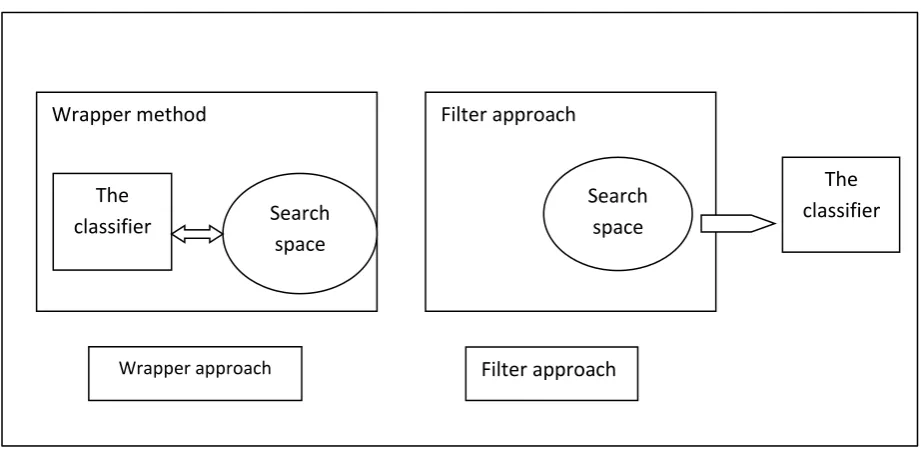
Subset evaluation is the process of checking whether each subset candidate is good enough. According to some evaluation criteria, the process of subset evaluation falls into two groups: wrapper and filter methods. In the wrapper method, the classifier itself is used to evaluate which subset of the features is more predictive, eliminating the one which is less predictive (Kohavi & John, 1997). In this technique, the classifier as the black box is considered part of the searching process, taking the feature subset and evaluating its accuracy using cross-validation evaluation; in turn, another subset enters the evaluation process until the most suitable subset in induced (Blum & Langley, 1997; John, Kohavi, & Pfleger, 1994). The idea of the wrapper approach is shown in Figure 2.1(Hall, 1999b). This process is claimed to be computationally expensive as the learning algorithm itself undertakes the responsibility of finding the best subset; on the other hand, however, the positive aspect is that it reduces the algorithm bias because the same classifier, which is used in the searching process, will be used later on in the learning. In the filter method, data will be characterised by itself, independently from the learning algorithm. The feature selection problem, in this case, totally depends on the data characteristics, its correlation, its dependency, and many other data evaluation criteria. The main disadvantage of this approach is that it ignores the effect of the inducer in the feature selection process; however, it is more adaptable when different classifiers are learnt for the same dataset as a result of not using the learning algorithm in the feature searching process. Nonetheless, its advantages outweigh its disadvantages (John et al., 1994):
Reduced computational costs as less data is involved in the learning process. Adaptable to any changes in the learning algorithm.
Much faster scaling to a large data set than the wrapper algorithm, as it can be re-run many times.
25 given, and the user should specify how many features are suitable for a specific learning process (Hall, 1999b). The filter approach concept is shown in Figure 2-1
Figure 2-1: Wrapper and Filter methods (Hall, 1999b)
3. Stopping criteria
Feature selection has to decide when to stop searching through the feature space, which depends on the evaluation criteria. Some of the used stopping criteria are as follows: Adding or removing features that do not add any value to the learning process (they
do not change the learning performance)
Reaching a specific stop pre-defined point, which includes:
o Whether a predefined subset is selected or a predefined number of iterations is reached (Dash & Liu, 1997)
o The result is ‗good enough‘
o Whether a specific number of features are selected
o No changes in the evaluation performance if feature is added or removed.
Filter approach
The classifier Search
space
Filter approach Wrapper method
Search space The
classifier
26 2.3.2 Feature Selection Literature Review
The first pioneer works in feature selection were carried out by Almuallim & Dietterich (1991) and Kira & Rendell (1992), both of which used the filter approach in two different ways. The former defines the FOCUS algorithm, which starts with an empty set and uses the breadth-first search strategy to establish the good enough solution by choosing the minimal subset that can be used to determine the label value for all instances in the training set, whereas, Kira & Rendell (1992) defined the RELIF algorithm which assigns a weight to each feature and accordingly finds the good enough feature that exceeds a user threshold. These two researchers assumed Boolean attributes, whereas Kononenko (1994) reports extensions to their methods that handle non-Boolean attributes and multiple classes. Other recent works rely on the wrapper approach rather than the filter approach. As mentioned before, the main argument of using the wrapper method is that the inducer itself is used in the feature selection process, which will reduce induction bias, rather than using two different isolated strategies: one for feature selection and one for induction (as is the case in the filter approach). The first pioneer work that uses the wrapper approach in the feature selection problem was that by John et al. (1994), where a decision tree is used to establish the ―good enough‖ feature subset. The simplest way to do this is to run the learning algorithm in a chosen feature subset and accordingly calculate the accuracy, then return back to introduce another subset that is either removed if it is worse or added if it is better. Various other attempts are carried out to replace the decision tree, used in the wrapper methods by other induction algorithms, such as (Aha & Bankert, 1994; Blum & Langley, 1997), both of which used a nearest neighbour algorithm within the wrapper algorithm. Likewise, Skalak (1994) works with the same concept but replaces greedy search with hill-climbing search.
27 There is a wealth of research comparing different feature selection approaches in different applications. Hall & Homles (2003) performed a benchmark comparison of several attribute selection methods for two supervised classification learning schemes, C4.5 and naive Bayes. Both studies show that different feature selection methods perform differently in different cases which conclude no best methods for all cases and emphasizes on the need of an approach to know in advance which is best for a specific task.
In this work, the importance of feature selection exists in exploring the type of feature selection method most suited to a specific type of data, and which are far from its learning scope. Thus, this is the aim of the process, where a direct connection will be carried out between feature selection methods and dataset characteristics with the aim of establishing which algorithm performs best if a specific feature selection method is carried out over a specific type of data.
2.3.3 Feature Selection in Meta-learning Work
The literature search did not reveal any use of meta-learning for feature selection, other than its use for reducing the number of meta-features by Kalousis & Hilario (2001) and Todorovski, Brazdil, & Soares (2000). In the first work, a feature selection wrapper method is used to make a pairwise comparison. In this comparison, the relative performance of each pair of base learners is contrasted using different meta-learners after removing irrelevant meta-features using feature selection methods. The result shows the importance of using feature selection in the meta-level process. In the second work, feature selection methods are used to remove irrelevant features in meta-level learning. In the first step, when a new dataset emerges, a similar dataset from the meta-knowledge is found using k nearest point by calculating the nearest distance between two datasets using their attributes values, then the predicted new label for the new data is calculated to be the average of performance of each k nearest points found in the meta-knowledge. The performance for both before and after using feature selection in the meta-level process shows that choosing the relevant meta-feature has a potential effect on meta-learner predictive power.
28 time, effort and considerable experimentation. Hence, this thesis will also explore the use of meta-learning for feature selection.
The next section covers active learning and its application in data mining process.
2.4 Active Learning
Active learning is a subfield of machine-learning, where the learning algorithm is given the ability to choose the data from which it learns with the aim of making the learner perform better with less training examples. The learning algorithm in active learning has control over the input data in its learning process (Cohn, Atlas, & Ladner, 1994; Lindenbaum, Markovitch, & Rusakov, 2004; Tong & Koller, 2002). This is a very practical way of reducing the costs needed to label all training examples whilst eliminating some degree of redundancy in the information content of the labelled examples. Active learning is well-motivated in many modern machine-learning problems, where unlabelled data may be abundant or easy to obtain, such as in the case of unlabelled webpages available in thousands of pages; however, labels are difficult, time-consuming or expensive to obtain, such as classifying each web page as ‗relevant‘ or ‗not relevant‘ to web users. It has been shown that less than 0.0001 % of all web pages have topic labels (Fu, Zhu, & Li, 2013); therefore, having to label those thousands of web pages would be very time-consuming. Another example is detection of fraud in banks, where an expert in a bank needs to invest considerable effort and time to label a bank customer‘s behaviour as fraudulent or not fraudulent.
29 2.4.1 Active Learning Background
This section sheds light on the main directions of using active learning in machine learning and provides a background on this topic and in using active learning for meta-learning.
Active learning is best defined in contrast to passive learning: in passive learning, a learner has access to the initial randomly generated labelled examples to build a hypothesis that covers most of the training data. In the traditional learning process (passive learning), the more labelled training data that is available, the more accurate the classifier that will be developed (Prudancio & Ludermir, 2007). In most learning problems, having a labelled (classified) example is not an easy process; this needs time and effort. Therefore, developing a strategy that conducts a classification process with the least possible labelled data is the main aim of active learning. The active learning model is a slightly different framework than other learning frameworks in which a small number of available initial data has labels, whilst a large amount does not come with any labels; that is, most of the training data set is simply an input without any associated label. The goal of active learning is to seek more unlabelled examples for labelling but those unlabelled example should have specific condition to say that they are ‗informative enough‘ to be allowed to enter the labelling process. The term ‗informative‘ is defined in active learning using different methods and different strategies. The following presents an overview of active learning scenarios and methods.
2.4.1.1 Active Learning Scenarios
There are many scenarios in which active learning can be used. The main three scenarios found in the literature are described here: (1) membership query synthesis, (2) stream-based selective sampling, and (3) pool-based sampling.
1. Membership Query Synthesis
30 2. Stream-based Selective Sampling
In the stream selective sampling, instances are drawn from actual data distribution, with the learner then deciding whether to include or discard it from the learning process. This approach, in some studies, is known as stream-sampling or selective sampling (Settles, 2011) because instances are selected one by one to enter the learning process.
3. Pool-based Sampling
This scenario is the most widely used scenario in active learning problems. In this scenario, the learner considers that there is a small pool of labelled examples and a large pool of unlabelled examples. Each time a query is applied on an unlabelled example, the most informative (or best) unlabelled example is chosen to be labelled, this includes starting with a large pool of unlabelled examples, picking a few points for labelling, then querying for more instances to be labelled in many different ways. Below is the active learning process for the pool-based sampling scenario (Melo , Hannois , Rodrigues , & Natal 2011) :
Start with a large pool of unlabelled data Pick a few points at random and get their label Repeat the following:
1. Fit a classifier to the labels seen so far
2. Pick the BEST unlabelled point to get a label for: i. Closest to the boundary.
ii. Most likely to decrease classifier uncertainty.
iii. Most likely to reduce the overall classifier error rate.
iv. High disagreement between learners (in the case of more than one classifier) on how to label it.
v. Most likely to reduce variance and bias.
31 in the stream-based sampling scenario comes as stream, with the learner then evaluating each query one by one, and accordingly deciding whether to accept or discard the data. In our work, we will use the pool-based sampling.
In this scenario, deciding which data is more informative is known as query strategy. Below is a description of the different query strategies found in the literature.
2.4.1.2 Active Learning Query Strategy
In the literature, several methods have been used to query the most informative data for labelling. Different query strategies are described below.
1. Uncertainty Sampling
Uncertainty sampling is the most common search strategy used in active learning. In some studies, it is known as query by uncertainty or uncertainty reduction. In this strategy, the pre-built classifier (the classifier that was built from the small pool of labelled data) is less confident in terms of how to classify the labelled data; those are the data that are nearer to the classifier boundaries. As a conclusion, if data uncertainty is high, this implies that the current model does not have a sufficient knowledge in how to classify it, thus meaning it is most likely that including such data in the learning process will improve model performance. This strategy is used in different machine-learning fields, such as natural language processing (Lewis & Gale, 1994), and in different classifiers: decision tree (Lewis & Gale, 1994), support vector machine (Tong & Koller, 2002) and in nearest-neighbour classifier (Lindenbaum et al., 2004). The key point in this approach is how to evaluate uncertainty measurements.
32 2. Error Reduction
This method depends on the estimation of how much classification error is likely to be reduced using the new dataset (Cohn, Ghahramani, & Jordan, 1996; Zhu, Lafferty, & Ghahramani, 2003).
3. Variance and Bias Reduction
This method depends on selecting samples that reduce learner bias and variance, which can be done by applying two learners: the single learner, such as naive Bayes, and bagging using naive Bayes as its base learner (or any other ensemble techniques), then asking the active learner to choose the informative data that reduces the difference between prediction using the first learner and the second learner (Aminian, 2005).
4. Outlier Detection
Most of work carried out on active learning considers the data around the decision boundaries, as explained above (uncertainty sampling), although it is worth pointing out here that the uncertainty sampling technique fails to detect outliers. Outlier data is highly uncertain but does not provide any help in the learning process because outlier data is defined as an observation that deviates too much from other observations, and also does not provide any extra knowledge if they enter the learning process.
33 5. Query-By-Committee
Query by committee is a very effective active learning approach used in many classification problems (Cohn et al., 1994; Melville & Mooney, 2004; Seung, Opper, & Sompolinsky, 1992). It is the same as the query by uncertainty method, although the main difference between query uncertainty sampling and query by committee is that query by committee is a multi-classifiers approach where more than one classifier is imposed upon the original labelled data set. The more there are disagreements on how to
A 1
B 1
[image:42.595.73.504.248.475.2]Unlabelled data Labelled data
34 classify a piece of data, the more informative the data. The idea behind this strategy is that enables classification strategy, where different classifiers should agree, to a high extent, on classifying new instances (by voting or averaging). In active learning, the disagreement gives new instances the favour of being chosen to enter the new classification process (Melville & Mooney, 2004) because this disagreement means that the classifier (set of classifiers) is not sure (not certain) on how to classify it, which emphasises the uncertainty sampling concept.
6. Sampling by Clustering
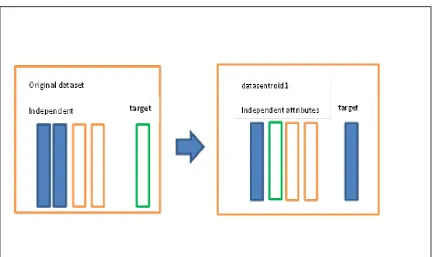
In previous methods, the labelled data used to build the first learner is chosen randomly with the assumption that they have some prior data distributions; in most cases, however, this assumption is not correct due to the small size of initial data chosen, meaning it is most likely they are not a good representative for the whole dataset. For the aim of solving this problem, some researchers suggest clustering the whole dataset and then choosing the data that is more representative. Such data are the data that are nearer to the initial clusters‘ centres (Nguyen & Smeulders, 2004; Xu, Yu, Tresp, Xu, & Wang, 2003; Zhu et al., 2008a). In the work of (Zhu, Wang, Yao, & Tsou, 2008b), all unlabelled examples are clustered first, and data that are around the centre are taken to form the first set of labelled examples. Subsequently, more informative data are queried from unlabelled data using uncertainty sampling and density measures, as described above. Another work adopted active learning by clustering (Nguyen & Smeulders, 2004), in which active learning using clustering is developed so that data from the same cluster is given the same label, which reduces the efforts needed to label all data in the same cluster. In the study of (Xu et al., 2003), the active learner measures uncertainty sample for the data around boundaries, then clusters those (uncertain) samples to query the most representative points around the cluster centre for text classification problems.
2.4.2 Active Learning in Meta-learning Scenarios