International Journal of Emerging Technology and Advanced Engineering
Website: www.ijetae.com (ISSN 2250-2459, ISO 9001:2008 Certified Journal, Volume 6, Issue 5, May 2016)
322
A Normalization scheme for Terrestrial LiDAR Intensity
Data by Range and Incidence Angle
Sandeep Sasidharan
Abstract— Automatic registration, classification and segmentation of Terrestrial Laser Scanner (TLS) data are of great interest in Geoinformatics & Autonomous vehicle research. Along with dense and accurate 3D geometric data, laser scanners also collect return intensity information. Inclusion of this spectral information has potential to improve the working of the above mentioned processes. However, these intensity values need to be normalized, prior to their use, as they are subject to a large number of errors. This paper presents a technique to carry out normalization of intensity values using the range and incidence angle corrections. The developed approach has been tested on a large number of data and results are found satisfactory.
Keywords— Terrestrial Laser Scanner, LiDAR, Intensity, Normalization, Incidence angle correction
I. INTRODUCTION
Terrestrial Laser Scanners (TLS) are capable of generating dense and accurate three dimensional data of object surfaces in a short period of time. In most cases the return intensity value for each point is also determined along with the 3D co-ordinates. This spectral information can be effectively incorporated into the existing LiDAR data processing algorithms, like registration, classification and segmentation, to obtain more accurate and faster results.
In the recent times there has been a surge in using intensity value as an additional information. Modern laser scanners are, therefore, having better intensity measurement. The return intensity from an object depends on the incidence angle of the laser on the surface, the surface properties and the laser wavelength [2]. Pfeifer et al. (2007) [5] studied the influence of varying the incidence angles and material reflectance properties on the return intensity. The experimental results presented by them show that the range dependent inverse-square model might not be sufficient to estimate the accurate intensity of the received laser pulse. Hence an empirical data driven model is proposed, which uses predefined homogeneous areas to empirically estimate the best parameters for global correction function by accounting for all influences from range, reflectance and incidence angle. Höfle and Pfeifer (2007) [1] also propose a model driven method for Airborne Laser Scanner (ALS), which corrects the intensities independently based on physical principles of radar systems, for spherical, topographical and atmospheric influences.
Gross et al. (2008) normalizes the value of the airborne laser scanner intensity data by considering the incidence angle derived by the sensor and object position as well as its surface orientation.
Pesci and Teza (2008) [4] studied the effects of surface irregularities on the intensity data captured by Terrestrial Laser Scanner. From a series of experiments they were able to conclude that the intensity of the signal backscattered by a planar element decreases if the incidence angle increases, whereas the intensity of the signal backscattered by the irregular surface is almost constant if the incidence angle varies. In our approach, the huge point cloud data captured by TLS is clustered into small data clouds representing homogenous regular surfaces. Statistical score normalization process using z-scores were implemented for intensity normalization by Hefford and Samson (2009) for point cloud registration of data collected from 2D laser scanners of mobile systems, assuming that the intensity data follow normal distribution. Considering the significance of intensity normalization this paper presents a methodology, by using and modifying the existing knowledge, to implement intensity normalization and presents the results thus obtained to show success of the proposed method. A preliminary version of the methodology proposed with only a few results was presented at INCA conference [6] and discusses in [9]. This paper is extension of this work with fully developed methodology and a large number of results to validate the methodology.
II. THEORETICAL BACKGROUND
The intensity information collected by a laser scanner is subject to a large number of errors due to atmospheric losses, sensor noise, hardware sensitivity, laser wavelength, surface geometry of the target etc. In the case of terrestrial laser scanners, the distance of the scanner from the target as well as the incident angle of the laser pulse on the target are the most important factors to be considered for the anomaly in the recorded intensity values.
According to Wagner et al. (2006) [7], the recorded intensity is proportional to the range „R‟ raised to „n‟, where the value of „n‟ depends on the surface type of the target.
International Journal of Emerging Technology and Advanced Engineering
Website: www.ijetae.com (ISSN 2250-2459, ISO 9001:2008 Certified Journal, Volume 6, Issue 5, May 2016)
323 n ref act raw norm R R I
I
(1)
Where, Iraw = recorded intensity
Ract =actual distance between the laser instrument and the return
Rref= reference distance either determined by examining the distribution of Ract from all returns or specified arbitrarily by the user. For all point on planar surfaces, the intensity value is inversely proportional to the cosine of the angle of incidence (Gross et al., 2008) and can be represented by Equation 2. ) cos(i I I raw
norm (2)
Where, Iraw = recorded intensity Inorm= normalized intensity
i = incidence angle
In this paper the intensity normalization is applied assuming that the intensity characteristics of the LiDAR can be modeled. The reflecting surfaces are assumed to be homogeneous. Kaasalainen et al. (2007) [3] suggests a value of n=2 for homogenous targets filling the full pulse foot print, n=3 for linear objects, and n=4 for individual large scatterers. Hence combining Equation 1 and Equation 2, an equation for correcting the intensity data, for homogenous targets, with respect to range and incidence angle can be formulated as given in Equation 3. ) cos( 1 2 i R R I I ref act raw
norm (3)
III. INTENSITY NORMALIZATION
The ILRIS 3D equipment, used in this work, collects intensity data in two channels. While parsing the data, a user can select either 16 bit raw intensity format or 8 bit truncated grey intensity format or both. The intensity value recorded by the TLS is altered by the receiving optics, the hardware and the internal propriety software.
Figure1: Flow chart for Intensity Normalization Algorithm
The intensity directly provided by the instrument is called raw intensity. The 8 bit intensity data is derived from the raw intensity after applying some corrections and scaling these values to 8 bit format. The 16 bit to 8 bit intensity data conversion algorithm is applied by the instrument's internal propriety software for improving the visual quality of the point cloud and is not available to the end user. In this paper the terminology „raw intensity‟ refers to the 16 bit intensity data provided by the TLS. All the computations are performed assuming the TLS is stable and the behaviour of intensity values can be characterized.
OUTLIER REMOVAL
CLUSTERING LOCAL AREA FOR EACH POINT
LOCAL SURFACE FITTING
COMPUTING SURFACE NORMAL DIRECTION FOR POINTS
COMPUTING LASER PULSE DIRECTION FOR SURFACE POINTS
INCIDENCE ANGLE CALCULATION FOR EACH LASER PULSE
APPLYING RANGE AND INCIDENCE ANGLE CORRECTION
RAW POINT CLOUD DATA
International Journal of Emerging Technology and Advanced Engineering
Website: www.ijetae.com (ISSN 2250-2459, ISO 9001:2008 Certified Journal, Volume 6, Issue 5, May 2016)
324 As discussed, the LiDAR intensity values tend to show an anomaly for the same target material captured at different locations. The intensity normalization is performed in order to make the intensity values comparable of similar materials captured at different locations. Intensity normalization is a multistep procedure. The main routine involves finding the incidence angle for each laser ray at its point of interaction on the object surface and then applying the correction. The range correction is also applied simultaneously. The process flow is summarized as a flow chart in Figure 1.
Outlier Elimination
Before applying the normalization procedure, outliers must be removed from point cloud data. In the proposed algorithm, Delaunay Triangulation is employed to eliminate the outliers. A 3D TIN Delaunay Triangulation is performed for a pre-determined threshold value. The sides of the triangles having a length greater than the threshold are removed. This task can also be performed with the help of any 3rd party software package.
Clustering Local Area for Data Points
A simple k-nearest neighbour ball search is employed for clustering the data. For each data point the neighbouring data points, i.e., those lying within a user specified radius, are selected. The radial distance for the nearest neighbour ball search algorithm is a user specified value which depends on the point density of the scan. A method for automatic determination of this radius will be taken up as a future work.
Surface Fitting and Determining Normal Direction
To apply the incidence angle correction at each data point, the direction of the incident ray vector and the surface normal at each data point needs to be calculated. For individual clusters formed by each data point, a second order polynomial surface is fit and the direction of the surface normal at that data point is determined.
2 20 2 02 11 10 01 00 )
(z p p x p y p xy p x p y
f (4)
Where, f (z) represents the surface pij represents the equation co-efficient
A second order surface is preferred as it is expected that most of the surfaces in artificial objects are planar and also higher order surfaces are not common.
Equation 4 represents the fitted surface mathematically. The direction of the surface normal at a point (x,y,z) can be determined by finding the gradient of the surface function and substituting the values of x, y and z.
Computing Incidence Angle
The direction of the laser pulse can be computed for a point on the object provided the initial position of the scanner is known. Usually for Optech ILRIS36D the
origin is set to (0,0,0) at the fixing bolt. Cosine of the incidence angle i can be calculated by taking the ratio of dot products of direction of surface normal and the direction of the laser pulse at a particular point, as shown in Equation 5.
| || |
. cos1
dl dn
dl dn
i (5)
where,
dn
= direction of surface normald
l
= direction of laser pulseApplying Corrections
The normalized intensity now can be computed using the equation 3.
IV. INTENSITY NORMALIZATION RESULTS
The point clouds of the same materials captured at different scan locations are used for this analysis. Six sets of data are subject to normalization. The raw 16 bit intensity values obtained after parsing the scan data are used for normalization.
The intensity normalization results are shown in Table 1 along with mean and standard deviation (SD). The term 'Raw' and 'Norm' used in the table are for raw intensity and normalized intensity, respectively.
International Journal of Emerging Technology and Advanced Engineering
Website: www.ijetae.com (ISSN 2250-2459, ISO 9001:2008 Certified Journal, Volume 6, Issue 5, May 2016)
325
Table 1:
Intensity Normalization Results
Data Set No Material Scan No No of Points Raw Mean Raw SD Norm Mean Norm SD
1 Brick Wall-I Scan 1 30293 3290 622 44 8
Scan 2 30247 4365 778 53 9
2 Brick Wall-II Scan1 30247 4365 778 53 9
Scan 2 24625 1728 361 67 14
3 Concrete Wall-I Scan1 7368 418 192 104 48
Scan 2 4328 1385 505 147 53
4 Concrete Wall-II Scan1 1976 406 200 120 60
Scan 2 998 1070 603 136 68
5 Iron Door Scan1 7128 1900 284 34 5
Scan 2 998 6205 206 30 4
6 Plastic Object Scan1 11976 2186 441 36 7.5
[image:4.595.76.524.158.630.2]Scan 2 11312 1805 553 31 7.9
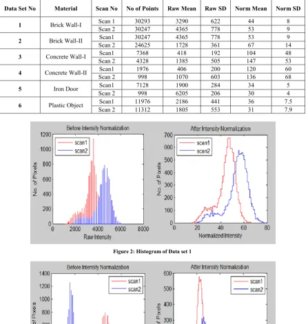
[image:4.595.118.474.537.718.2]Figure 2: Histogram of Data set 1
International Journal of Emerging Technology and Advanced Engineering
Website: www.ijetae.com (ISSN 2250-2459, ISO 9001:2008 Certified Journal, Volume 6, Issue 5, May 2016)
[image:5.595.115.480.122.740.2]326
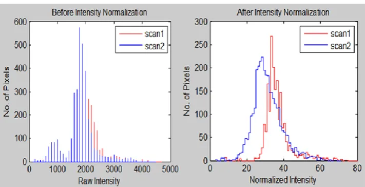
[image:5.595.121.476.134.311.2]Figure 4: Histogram of Data set 3
Figure 5: Histogram of Data set 4
[image:5.595.121.477.537.719.2]International Journal of Emerging Technology and Advanced Engineering
Website: www.ijetae.com (ISSN 2250-2459, ISO 9001:2008 Certified Journal, Volume 6, Issue 5, May 2016)
[image:6.595.117.517.130.328.2]327
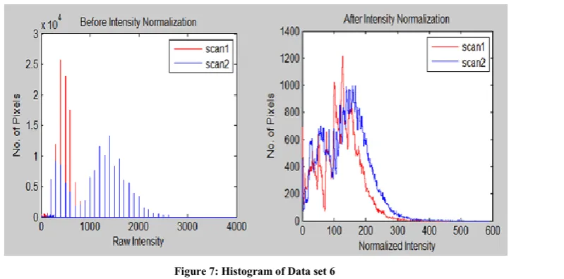
Figure 7: Histogram of Data set 6
Discussion on Intensity Normalization results
The raw intensity values, after incidence angle and range correction appeared to have comparable values for mean and standard deviation for both scans. Hence it can be inferred that after intensity normalization, intensities for the same material appear to have similar mean and standard deviation values and thus can be effectively incorporated as one of the enhancement parameters for any point cloud processing algorithm.
In order to quantify the results, the distance between the distributions is calculated using Equation 6.
j i j i
cos1 (6)
Where,
= distance co-efficient for the distribution
= mean of the intensity values
= standard deviation of intensity valuesi, j = scan numbers
The calculated distance between the distributions are tabulated in Table 2
Table 2:
Distance between distributions
Data Set Raw Normalized
Set 1 0.77 0.53
Set 2 2.31 0.61
Set 3 1.39 0.43
Set 4 0.45 0.44
Set 5 0.83 0.13
Set 6 0.39 0.32
Since LiDAR intensities are assumed to follow normal distribution, Hellinger‟s distance can be used for quantifying the similarities between the samples. Hellinger‟s distance can be calculated using Equation 7.
2 2 2 1 2 2 1 ) ( 4 1 2 2 2 1 2 1
2( , ) 1 2
e Q P
H (7)
Where, H is the Hellinger‟s distance P and Q = are the distributions
= mean of the intensity values
= standard deviation of intensity valuesi, j = scan numbers
Table 3 summarizes the Hellinger‟s distance between the intensities of scan 1 and scan 2 for each data set for raw and normalized intensities.
Table 3:
Hellinger’s distance between the intensities of scan 1 and scan 2 for each data set for raw and normalized intensity values.
Data Set Raw Normalized
Set 1 0.5117 0.3652
Set 2 0.958 0.4481
Set 3 0.7963 0.2978
Set 4 0.3410 0.3226
Set 5 0.6416 0.1078
Set 6 0.2858 0.2279
After intensity normalization, the distance between the intensity distributions of the scans is smaller compared to the raw data. This implies that the intensity value distributions are closer when normalized, thus proving that the suggested approach is able to make the intensities of two scans similar despite their different locations.
V. CONCLUSION
International Journal of Emerging Technology and Advanced Engineering
Website: www.ijetae.com (ISSN 2250-2459, ISO 9001:2008 Certified Journal, Volume 6, Issue 5, May 2016)
328 Even though some software provide automatic option, usually it is not preferred as it often produces undesirable results and consume large amount of primary memory. The use of intensity values can improve working of these algorithms. However, prior to use, the intensity values need to be normalized. This paper has presented a complete approach for intensity normalization and successfully shown the results using six different data sets. The proposed scheme results in bringing two different scans of same object closer in terms of their radiometric characteristics. More importance is given to developing a simple, accurate and efficient algorithm. Further work will involve automatic determination of a few thresholds used in this paper and testing the algorithm on data from multiple scanners using different wavelengths and for different types of objects.
Note: This work was performed when the author was a Graduate Student at Indian Institute of Technology Kanpur, India
REFERENCES
[1] Höfle, B., & Pfeifer, N. 2007. Correction of laser scanning intensity data: Data and model-driven approaches. ISPRS Journal of Photogrammetry and Remote Sensing, 63(6), 415-433. [2] Jelalian, A. 1992. Laser Radar Systems. Artech House,Boston,
MA.
[3] Kaasalainen, S., Hyyppä, J., Litkey, P., Hyyppä, H., Ahokas, E., Kukko, A., & Kaartinen, H. 2007. Radiometric calibration of ALS intensity. IAPRS Volume XXXVI, Part 3 / W52, 2007, ISPRS
Workshop on Laser Scanning 2007 and SilviLaser 2007, Espoo, September 12-14, 2007, Finland
[4] Pesci, A., & Teza, G. 2008.. Effects of surface irregularities on intensity data from laser scanning: an experimental approach. Annals of Geophysics, 51(5/6).
[5] Pfeifer, N., Dorninger, P., & Fan, H. 2007. Investigating terrestrial laser scanning intensity data: quality and functional relations. In: Gruen, A., Kahmen, H. (Eds.) International Conference on Optical 3-D MeasurementTechniques, VIII, 328-337.
[6] Lohani, B., & Sasidharan, S. 2012. Intensity Augmented ICP for Registering Laser Scanner Point Clouds. Proceedings of XXXII INCA International Congress on Cartography for Sustainable Earth Resource Management, Indian Cartographer, Vol. XXXII, pp 30-34.
[7] Wagner, W., Ullrich, A., Ducic, V., Melzer, T., & Studnicka., N. 2006. Gaussian decomposition and calibration of a novel small-footprint full-waveform digitizing airborne laser scanner. Journal of Photogrammetry and Remote Sensing, 60, 100-112.
[8] Lohani, B., Chacko, S., Ghosh, S., and Sasidharan, S.“Surveillance system based on Flash LiDAR.” Proceedings of XXXII INCA International Congress on Cartography for Sustainable Earth Resource Management, Indian Cartographer, Vol. XXXII, pp 77-85 September 17, 2013.