ABSORPTION GRATING DIFFUSERS
Konstantinos DADIOTIS
School of Computing, Science and Engineering
University of Salford, Salford, UK
Submitted in Partial Fulfilment of the Requirements of the
with Pan (god of shepherds and flocks), he caused confusion in nearby shepherds that led them to kill her and tear her to pieces which they scattered throughout the land. Gaea (Earth) out of mercy collected the scattered pieces which she buried where she found them. However, the pieces kept her godly melodic voice. Thus, she remains scattered throughout
FIGURE CAPTIONS...V
SYMBOL AND ABBREVIATION INDEX... XIV
ACKNOWLEDGEMENTS... XVII
ABSTRACT...1
INTRODUCTION...3
PART I. PHASE GRATING DIFFUSERS...5
CHAPTER 1. INTRODUCTION TO DIFFUSERS ...7
1.1. Measures of diffusion ...7
1.1.1. Scattering coefficient...? 1.1.2. Diffusion coefficient... 8
1.1.3. Discussion... 9
1.2. Sequences... 9
1.2.1. 1-D sequences... 10
1.2.2. 2-D sequences... 10
Superimposing a 1-D sequence on 2 dimensions... 10
Chinese Remainder Theorem ... 11
Changing the folding steps in the Chinese Remainder Theorem ... 13
1.3. Summary... 14
CHAPTER 2. ASSESSING A DIFFUSER... 15
2.1. Prediction methods ... 15
2.1.1. Boundary Element Modelling (BEM)... 15
Thin panel Boundary Element Modelling ... 18
Far-Field... 20
2.2. Scattered pressure distribution measurement methods... 21
2.3. Measurements Vs Simulations... 24
2.3.1. Boundary Element Modelling ...25
2.3.2. Fourier Model... 26
2.3.3. Discussion... 28
2.4. Summary... 28
CHAPTER 3. STANDARD PHASE GRATING DIFFUSERS ...29
3.1. The diffusers ... 29
3.2. Disadvantages... 32
3.2.1. Flat plate frequencies... 32
3.2.2. Well cut-off frequencies limitations... 33
3.3. Periodicity... 33
3.4. Modulation... 36
3.4.1. Using the inverse of the base sequence:... 36
3.4.2. Using the base sequence in reverse order:... 37
3.4.3. Using a different sequence to that of the base diffuser: ... 37
3.5. Diffusion... 38
3.6. Summary... ...-40
CHAPTER 4. NEW SEQUENCES FOR PHASE GRATING DIFFUSERS
...41
4.1. Power Residue Sequence Diffusers (PWRD)...41
4.1.1. The sequence ...42
4.1.2. The diffusers...46
4.2. Luke Sequence Diffusers (LSD)...-...-... 58
4.2.1. The sequences...-... ... ... 59
4.3. Discussion... 67
4.4. Further Suggestions ... 68
4.4.1. Using half a QRD or PRD instead of the full one ... 68
4.4.2. Folding PRD forming parallel PWRDs... 69
4.5. Summary... 71
PART II. ABSORPTION GRATING DIFFUSERS ...72
CHAPTERS.
INTRODUCTION
TO
ABSORPTION
GRATING
DIFFUSERS
...73
5.1. Introduction... 73
5.2. Advantages and Disadvantages... 75
5.3. Reasons for Doubt ...76
CHAPTER 6. ABSORBERS...79
6.1. Measures... 79
6.2. Prediction models ... 80
Transfer Matrix Model... 81
Prediction models of the characteristic properties of a porous material... 82
6.3. Impedance tube measurements ... 83
6.3.1. Surface impedance measurement... 83
6.3.2. Measurement of characteristic properties... 86
6.4. Types of absorbers...-.---...-..---...-..--- 90
6.4.1. Layer of porous materials...-.---—... —.-—90
6.4.2. Helmholtz Resonators ...91
Loaded Helmholtz Resonators...—...— .. — . — ... 94
6.5. Summary...—... — ...——.——.—..••••••••••••••••••••••••••••••••••••••••••••••••••••••••••••97
CHAPTER 7. IMPLEMENTATION OF THE ABSORBING ELEMENTS
WITH PERFORATIONS ON A MASK...98
7.2. Helmholtz Resonator impedance tube measurements ... 99
7.3. Helmholtz Resonator BEM simulation... 102
7.4. Different perforation patterns ... 107
7.5. Summary... HI
CHAPTERS.
SCATTERED
PRESSURE
DISTRIBUTION
FROM
ABSORPTION GRATING DIFFUSERS ...112
8.1. Reflecting elements... 112
8.2. Ideally Absorbing elements ... 117
8.3. Distribution of admittance on a surface... 118
8.3.1. Pseudorandomly arranged ... 118
8.3.2. Periodic... 123
8.4. Discussion... 126
8.5. Summary... 126
CHAPTER 9.
IMPROVEMENTS
TO
ABSORPTION
GRATING
DIFFUSERS
...131
9.1. Reactive elements in the place of the reflective... 131
9.1.1. Helmholtz Resonators ... 131
9.1.2. Discussion... 135
9.2. Imperfect absorbing elements... 137
9.2.1. Measurements Vs Boundary Element Modelling... 137
9.2.2. Simulations... 140
9.3. Absorption in wells of Phase Grating Diffusers ... 146
9.3.1. Absorption in all the wells... 147
9.3.2. Absorption in all selected wells... 147
9.4. Discussion... — .-... — ...----.-. ——••• 148
CONCLUSIONS AND FURTHER WORK ...150
Figure 1-1. One period of a Maximum Length Sequence Diffuser (MLSD) of well width w
and depth of the n'h well, rfn ... 5
Figure 1-2. One period of a Quadratic Residue Diffuser (QRD) of well width w and depth of the n h well, dn ...5
Figure 1-1. Generating a 2-D sequence from a 1-D quadratic residue sequence... 11
Figure 1-2. From 1-D to 2-D QRD... 11
Figure 1-3. The positions of the coefficients of a 20-coefficient long sequence when folded in a 4x5 array using the Chinese Remainder Theorem... 12
Figure 1-4. Generating the positions of the coefficients of a 20-coefficient long sequence when folded in a 4x5 array using the Chinese Remainder Theorem throught the use of a space of parrallel arrays... 12
Figure 1-5. The positions of the coefficients of a 20-coefficient long sequence when folded in a 4x5 array with step\ = 2 and stepi = 3... 14
Figure 2-1. The Geometry of the boundary integral equation... 16
Figure 2-2. A plane surface meshed for a BEM... 17
Figure 2-3. Quadratic Residue Diffuser (QRD) geometry in the thin panel BEM... 19
Figure 2-4. Far-field determination... 20
Figure 2-5. Free-field equivalent of the semi-anechoic chamber...21
Figure 2-6. Single plane polar response measurement set-up in the semi-anechoic chamber. 22 Figure 2-7. Measured impulse responces with and without the sample... 23
Figure 2-8. Measured scattered impulse response of the sample... 23
Figure 2-9. Measured normal incidence scattered pressure distribution of a rigid surface 70cm wide at l.&kHz. ...24
Figure 2-10. Normal incidence scattered pressure distribution (dB) measurement Vs BEM prediction from a rigid surface, (a) IkHz, (b) 2kHz, (c) 4kHz and (d) 6kHz. ——— Measured, ——— Predicted... 25
Figure 2-12. Normal incidence scattered pressure distribution (dB) measurement Vs the Fourier Model prediction from a rigid surface normalized to the same sum of the reflected pressure, (a) IkHz, (b) 2kHz, (c) 3kHz, (d) 4kHz, (e) 5kHz and (f) 6kHz. ——— Measured,
—— — Predicted...^? Figure 3-1. One period of a Maximum Length Sequence Diffuser (MLSD) of well width w
and depth of the nth well, dn . ... ..29
Figure 3-2. One period of a Quadratic Residue Diffuser (QRD) of well width w and depth of then"1 well, dn .. ... ... ...29
Figure 3-3. Magnitude of autocorrelation function of a quadratic residue sequence (P=l).... 31
Figure 3-4. Reflection coefficients of a 1-D QRD (N = 7) at 1,2 and 4 (left) 3, 5, 6 (right) times the design frequency. ... 32
Figure 3-5. The flat plate effect of a QRD (P=7). ... 33
Figure 3-6. Lobing introduced by the constant patches of reflection coefficient when the width of the patches is equal to half of the wavelength (w/A = 1/2). ... 34
Figure 3-7. Lobing introduced by 3 periodic repetition of the diffusers when the width of a single diffuser is equal to two times the wavelength (W//1 = 2)... 35
Figure 3-8. Lobing introduced by the combination of constant patches of reflection coefficient and periodic repetition of the diffuser (Q = 3, N = 4, wlX = 1/2)... 35
Figure 3-9. Modulation of two PGDs using the binary sequence [1,0,1,1]... 36
Figure 3-10. The inverse of a QRD (P=7).... ... 36
Figure 3-11. The mirror of a PRO (P=7)... ... 37
Figure 3-12. Normalised diffusion coefficient Fourier Model prediction of 5 periods of QRD (p=7) with the design frequency set at 1 kHz ( •••• upper frequency limit). ... 38
Figure 3-13. Normal incidence scattered pressure distribution Fourier Model prediction of 5 periods of QRD (p=l) at the design frequency at/ = /0 = \kHz (a),/= 2/0 = 2kHz (b) and the flat plate frequency/= 7/o= 7^//z(c).. ... .39
Figure 3-14. The periodicity equivalent of 5 periods of a QRD... 40
Figure 4-1. PWRD (P = 11, M= 2, r = 0) generated from a PRO (P = 1 1)...42
Figure 4-2. Magnitude of autocorrelation function of all power residue sequences of period N = 9 that can be generated from different prime numbers. ... 43
Figure 4-21. Normal incidence scattered level distribution (dB) at the tilted Hat plate frequency of 2 periods of LSD (P = 42, r = 3) predicted using the Fourier Model (a) and
BEM(b)... 64
Figure 4-22. Diffusion coefficient, as predicted using the Boundary Element Model, of different types of periodic Luke and Primitive Root diffusers of the same total width... 65
Figure 4-23. BEM predicted normal incidence scattered level distribution (dB) at the flat plate frequency for 2 periods of LSD (p = 7, r = 1) periodic and modulated with its inverse in comparison with a plane surface of the same width...65
Figure 4-24. Normalised diffusion coefficient, as predicted using the BEM, of different modulations of LSD (P = 42, r= 1) of the same total width... 66
Figure 4-25. l/3rd octave band normalised diffusion coefficient, as predicted using the BEM, of different types of modulated diffusers, with their inverse, of the same total width... 67
Figure 4-26. Half a QRD used to form a full diffuser... 68
Figure 4-27. PRD (p=l) split into two half that are inverse of one another...69
Figure 4-28. The positions of the coefficients of a 20-coefficient long sequence when folded in a 4x5 array with the Chinese Remainder Theorem... 69
Figure 5-1. Autocorrelation function for a bipolar and a unipolar MLS(&=4) of period N = 15. ...74
Figure 5-2. 1-D Absorption Grating Diffuser constructed using a MLS (k = 3), sn = [0, 0, 1,0, 1,1,1]...^ Figure 5-3. Fourier theory equivalent of a AGD...76
Figure 5-4. BAD™ panel manufactured by RPG... 77
Figure 6-1. Sound reflection from through a surface...79
Figure 6-2. Geometry of the propagation of sound through a multi-layer medium... 81
Figure 6-3. Geometry of the propagation of sound through a single layer medium in front of a rigid backing... 82
Figure 6-4. Impedance tube setup for measuring surface impedance... 83
Figure 6-5. Square impedance tube with cross-section 5.4x5.4cm", ¥2 inch microphones positioned at x\ = 9.93cm and x2 = 15.03cm (frequency range 300//Z </< 3kHz)... 85
Figure 6-6. Impedance tube extension of adjustable depth with wooden termination... 85
Figure 6-7. Plate geometry... 86
Figure 6-9. Briiel & Kjaer 4206-T impedance tube kit for measuring characteristic impedance and characteristic wavenumber... 89 Figure 6-10. Impedance tube measurment of the characteristic impedance zc of black open cell foam... 89 Figure 6-11. Impedance tube measurement of the characteristic wavenumber kc of black open cell foam...90 Figure 6-12. Absorption coefficient of 5cm deep open cell estimated from its characteristic impedance and wavenumber. ...91 Figure 6-13. A Helmholtz Resonator and its mechanical equivalent... 92 Figure 6-14. Helmholtz Resonator with cavity volume V, hole-depth d and hole-radius a, morphed into a surface. ...93 Figure 6-15. Measured absorption coefficient in an impedance tube of a Helmholtz Resonator morphed into a surface with resonant frequency fr = 900Hz (cavity volume V = 38cm3 , hole- area S = 2cm 2 and hole-depth t= 1.5mm)...94 Figure 6-16. Periodically perforated surface backed by absorbing material in front of a rigid backing. ...95 Figure 7-1. The cross-section that is tested in the square impedance tube can be considered to be a single period of an infinitely wide surface... 99 Figure 7-2. Sample plates out of 1.5mm aluminium sheets... 99 Figure 7-3. Absorption coefficient of Helmholtz Resonators with the hole in the center of the sample of varying hole-diameters (d) for the same cavity volume (2.9x5.42cm3) and plate thickness (1.5mm)... 100 Figure 7-4. Measured normalised surface impedance of a layer of 29mm of layered mineral wool... 101 Figure 7-5. Absorption coefficient of Helmholtz Resonators with the hole in the center of the sample of varying hole-diameters (d) for the same cavity volume (2.9x5.42cra3) and plate thickness (1.5mm) loaded with layered mineral wool... 101 Figure 7-6. BEM prediction for uniform admittance distribution in the sample area. The input was the measured surface admittance of a Helmholtz Resonator with the hole in the center of the sample. ...•.•...•••••••••••••••••••••••••••••••••••• — ••••••••—— — — •••••••••• — •• 103 Figure 7-7. Absorption coefficient when all the admittance of the Helmholtz Resonator (d =
Resonator divided by the open area... 105 Figure 7-10. BEM prediction of the normalised surface impedance of a Helmholtz Resonator when only the hole-area in absorbing. The input is the measured surface admittance of a Helmholtz Resonator divide d with the open area... 106 Figure 7-11. Absorption coefficient of loaded Helmholtz Resonators of varying patterns of perforation for the same hole-diameters (16mm), cavity volume (2.9x5.42(V) and plate thickness (1.5mm)... 107 Figure 7-12. Absorption coefficient of the hole-area of loaded Helmholtz Resonators of varying patterns of perforation for the same hole-diameters (16mm), cavity volume (2.9x5.42cm3 ) and plate thickness (1.5mm)... 108 Figure 7-13. Normalised surface admittance of the hole-area of loaded Helmholtz Resonators of varying patterns of perforation for the same hole-diameters (16mm), cavity volume (2.9x5.42cm3) and plate thickness (1.5mm)... 108 Figure 7-14. Loaded Helmholtz resonators in two groups with samples in the same group having identical open area (top 3 lines - 28%, bottom 2 lines - 7%). ... 109 Figure 7-15. Same pattern emerging from different hole configurations... 110 Figure 8-1. BEM predicted diffusion coefficient of a flat plate of width w.... 113 Figure 8-2. BEM predicted mean reflected intensity (dB) in all the angles of reflection, in the specular and non-specular reflection zone from a flat plate of width w normalised to the incident pressure at the receiver that is normal to the surface... 114 Figure 8-3. BEM prediction of the normal incidence scattered level distribution (dB) from a flat plate of width w at A = w/4 (a),/I = 2w (b) and A = Ww (c)... 115 Figure 8-4. BEM predicted ratio of the mean reflected intensity in the non-specular over the specular zone of a plate of width vv... 116 Figure 8-5. BEM prediction of the normal incidence scattered level distribution (dB) from a flat plate of width w at the wavelength limits of applicability for AGDs Amax = 3w (a) and Amm = 0.83w(b)...»
Figure 8-6. BEM realisation of an absorbing surface of width w, normalised surface admittance of/?,, = 1 and rigid sides. ... 117
Figure 8-8. BEM prediction of the normal incidence scattered level distribution (dB), normalised to the specular lobe of a rigid surface, of a surface with reflecting elements arranged pseudorandomly with MLS (k = 5) at A = 31w (a), A = 3w (b), A = w (c) and A = w/2(d)... 119
Figure 8-9. BEM prediction of the normalised diffusion coefficient (dn ) and absorption
coefficient (ar) from a suface with reflecting elements arranged pseudorandomly using MLS
(fe = 5). ...120 Figure 8-10. Surface with reflecting elements arranged pseudorandomly using 4 periods of MLS (k = 3)... 121
Figure 8-11. BEM prediction of the normal incidence scattered level distribution (dB), normalised to the specular lobe of a rigid surface, of a surface with reflecting elements arranged pseudorandomly using 4 periods of MLS (k = 3) at A = 7w (a), A = 3w (b), A = w
(c) and A = w/2 (d)... 122 Figure 8-12. BEM prediction of the normalised diffusion coefficient (dn ) and absorption
coefficient (ar) from a suface with reflecting elements arranged pseudorandomly using 4
periods of MLS (k = 3)... 123
Figure 8-13. Suface with periodicly positioned reglective elements (of width W) positioned
every 2 W... 124 Figure 8-14. BEM prediction of the normalised diffusion coefficient (dn ) and absorption
coefficient (a r) from a suface with periodically positioned reflective elements (width W =
4w) positioned every 2W... 124
Figure 8-15. BEM prediction of the normal incidence scattered level distribution (dB), normalised to the specular lobe of a rigid surface, of a surface with periodically positioned reflective elements (width W 4w) positioned every 2 W at A = 7w... 125
Figure 8-16. BEM prediction of the pattern of the normal incidence scattered level distribution (dB) of a suface with periodically positioned reflective elements (width W = 4w) positioned every 2W at A = 2w in comparison with a single reflective element... 125
Figure 9-1. A Helmholtz Resonator formed in a 2-D surface... 131 Figure 9-2. 2-D Helmholtz Resonators geometry used in BEM... 132 Figure 9-3. BEM predicted non-specular over specular reflected level from a Helmholtz Resonator with a resonant frequecy at lr = 2w/3 compared to a plane surface of the same
Figure 9-4. BEM predicted normal incidence scattered pressure distribution from a Helmholtz Resonators with resonant wavelength 2w/3 compared to a plane surface of the same width w
at I = w/3 (a), X = 2w/3 (b) and 1 = w (c)... 134
Figure 9-5. 2-D BEM geometry of an Absorption Grating Diffuser generated from 4 periods of MLS (k = 3) implemented using Helmholtz Resonators in the place of the large reflective
elements... 135 Figure 9-6. BEM predicted normal incidence scattered pressure distribution (dB) from a Absrorption Grating Diffusers implemented using Helmholtz Resonators (Xr = 2w) compared
to a flat Absorption Grating Diffuser of the same dimensions at 1 = w/2 (a), X - Xr = 2w (b)
and /I = l\v (c), where vr is the width of smallest reflective element... 136
Figure 9-7. Absorption Grating Diffuser to be measured. The black parts consist of porous absorber and the brown ones of wood... 137 Figure 9-8. Absorption Grating Diffuser to be measured. The black parts consist of porous absorber and the brown ones of wood... 138 Figure 9-9. Normalised surface admittance of a 1.5cm deep leayer of black open cell foam
estimated from its characteristic impedance and wavenumber which were measured in an impedance tube... 139 Figure 9-10. Normal incidence scattered pressure distribution (dB) measurement Vs BEM prediction from an absorption grating surface generated by 4 periods of MLS(&=3) normalized to the same sum of the reflected energy, (a) IkHz, (b) 2kHz, (c) 3kHz, (d) 4kHz,
(e) 5kHz and (f) 6kHz. ——— Measured, ——— Predicted... 140
Figure 9-11. BEM prediction of the normalised diffusion coefficient (dn ) and absorption
coefficient (ar ) from an Absorption Grating Diffuser arranged using 4 periods of MLS (k = 3)
with the absorbing elements implemented by 7.5cm deep layer of foam... 141 Figure 9-12. Reflection coefficient of a 1.5cm deep leayer of black open cell foam estimated
from its characteristic impedance and wavenumber which were measured in an impedance
tube...^
Figure 9-13. BEM predicted normal incidence scattered pressure distribution from an absorption grating surface generated by 4 periods of MLS(fr=3) compared to a plane surface of the same width at/= 9007/z (a),/= L9kHz (b) and/= 2.8kHz (c)... 143
SYMBOL AND ABBREVIATION INDEX
Symbols
c speed of sound
d well depth
dc autocorrelation diffusion coefficient
dn normalised autocorrelation diffusion coefficient
E energy
/ frequency
/o diffuser design frequency
fr resonant frequency
G Green's function
h impulse response
H transfer function
H0 0th order Hankel's function
/ intensity
/ imaginary unit
k wavenumber
kc characteristic wavenumber
m mass
mod function that indicates the least non-negative remainder
M population of a family of sequences
p pressure
P, p sequence integer number generator
f position vector
rm losses
R reflection coefficient
RXX autocorrelation function
5 sequence
5 surface
T transfer matrix component
/ Helmholtz Resonator neck depth
/' Helmholtz Resonator neck depth including the radiation impedance
u particle velocity
V volume
H' well width
zc characteristic impedance
zn normalised surface impedance
zs surface impedance
a absorption coefficient
ar approximate absorption coefficient
ft surface admittance
/?„ normalized surface admittance
6 end correction
e open area
6 , y/ angle
/I wavelength
AO diffuser design wavelength
Xr resonant wavelength
p density
r delay
(p phase
ft) angular frequency
n, r, m, (, £ i counters
ACF Autocorrelation Function
AGD Absorption Grating Diffuser
BEM Boundary Element Modeling
LSD Luke Sequence Diffuser
MLS Maximum Length Sequence
MLSD Maximum Length Sequence Diffuser
PRD Primitive Root Diffuser
PGD Phase Grating Diffuser
PWRD Power Residue Diffuser
ACKNOWLEDGEMENTS
I would like to thank my family for their support throughout my studies. My parents Loukas and Petroula for their help and encouragement for success, my brother Dimitris for his advice and his help in my introduction to programming and my fiancee Georgia for the emotional support she provided and the patience she showed during my studies.
I am gratefully to the supervisory team of Prof. Cox and Prof. Angus for their help and guidance for the duration of my PhD studies. I feel I need to thank Prof. Cox in particular for his supervision of the completion of my research and the writing of this thesis.
I feel indebted to all the members of the Acoustics Research Centre of the University of Salford whether students or member of staff for the excellent cooperation and companionship. They made my experience of living and studying among them a memory that I will cherish forever.
I would like to thank in particular my colleague Richard Hughes for the excellent cooperation and the numerous hours of discussion on diffusers that stretched beyond the limits of the University.
Finally, I want to thank Dr. Peter D'Antonio for his advice on diffuser design.
I would also like to acknowledge the support of the Engineering and Physical Sciences Research Council, UK for funding this project through their Doctoral Training Account
This thesis investigates room acoustic diffusers based on number sequences, exploring their shortcomings and presents improvements.
Standard Phase Grating Diffusers display frequencies where they act like flat plates and fail to diffuse. To overcome this, two new sequences (Luke and power residue) are introduced. The diffusers based on these sequences display extended frequency range compared to standard ones such as Quadratic Residue and Primitive Root Diffusers. Their performance is studied using Boundary Element Modelling which shows that they can avoid flat plate phenomena in the audible frequency range. Furthermore, it is shown that by taking advantage of their inner symmetries Quadratic Residue and Primitive Root Diffusers can be created from smaller components thus allowing for the flat plat effect to be mitigated.
Next, Absorption Grating Diffusers are investigated. They consist of ideally absorbing and reflecting elements. For their implementation heavily damped Helmholtz Resonators are investigated showing that they give an approximation of the required distribution of admittance on the surface.
Then the performance of ideal Absorption Grating Diffusers is investigated using Boundary Element Modelling. Even with idealised completely absorbing elements, the performance of the diffuser is shown not to achieve substantial diffusion. This arises because edge diffraction from the reflecting elements weakens at high frequencies. At frequencies where smaller elements are creating substantial scattering, larger elements are producing specular reflections. Furthermore, due to the lack of cancellation, the specular reflected lobe is insufficiently attenuated, because it can only be changed through absorption.
Improvements to the original design are suggested. By changing reflective elements to reactive ones, scattering can be extended to higher frequencies. This allows for a range of frequencies were more reflecting elements display substantial dispersion. Also, implementing the absorbing elements using porous material in a shallow well allows some reflection, resulting in cancellation in the specular reflection lobe due to interference.
The acoustical quality of any performance space such as a concert hall, an auditorium, a club or a studio is the key factor in the perception of sound in it. For this reason these spaces are designed specifically for their application as they require different characteristics based on their use[l]. The sound field in a room consists of the interaction of the direct sound with the indirect reflections from its boundaries. The relationship between the amount of absorption on the walls and the sound decay of a room was established by Sabine[2] which launched modern room acoustic designfl].
The density and amplitude of the reflections dictates the acoustic characteristics of the space[3] and relates to its performance. The response of a boundary can be characterized in terms of absorption, reflection or diffusion. While the application of the right amount of absorption can be used to set the required reverberation time of a room[2] it does not necessarily take care of strong reflections from the boundaries of the room that can produce echo problems[4]. Furthermore, in cases that very little absorption is required in a small room there is need for diffusers to deal with the modal response of the space. Diffusers are structures whose main goal is to scatter the incident wave rather than attenuate it[5]. For this reason they can be used to deal with strong reflections from boundaries without removing sound energy from the space.
Diffuser research was ignited by Schroeder who suggested using number sequences to create diffusing surfaces[6]. Based on his concept, a category of diffusers was created known as Phase Grating Diffusers. Using the same mathematical approach Angus later presented the concept of Absorption Grating Diffusers[7] which are structures that combine the use of absorbing and reflecting elements to achieve diffusion.
In this thesis the characteristics of both Phase Grating and Absorption Grating Diffusers are investigated. The thesis is split into three parts:
common use. Boundary Element Modelling is used to predict their performance and compare them to commonly used Phase Grating Diffusers.
The second part of the thesis centres on Absorption Grating Diffusers. Their design concept is presented and their requirements are discussed. Porous absorbers and absorbing structures that can be used for their implementation are discussed along with measurement methods and analytical models that are used to assess their absorbing characteristics. The use of densely layered mineral wool behind a perforated structure is investigated as an implementation of highly absorbing elements. Boundary Element Modelling is used to investigate the absorbing and scattering capabilities of ideal Absorption Gratin Diffusers. Finally methods of improving their performance are introduced either by using reactive elements or by using less absorbing elements.
Phase Grating Diffusers (PGD) were invented in the 1970's by Manfred Schroeder, when he introduced the concept of using maximum length sequences to improve sound diffusion in concert halls and reverberation chambers[6, 8-10]. He suggested that by pseudorandom!y arranging wells of a constant depth on a surface (Figure 1-1) sound diffusion can be achieved[6]. This would be the case when the wave reflected out of the wells has opposite phase from the one reflected from the front surface.
Figure 1-1. One period of a Maximum Length Sequence Diffuser (MLSD) of well width w th
and depth of the n well, dn .
Based on the same concept Schroeder later suggested using wells of varying depth that would be dictated by integer based pseudorandom sequences such as quadratic residue (Figure 1-2) and primitive root sequences[8]. These diffusers were soon to become commonly used by the industry[5, 8, 11-12]. In 1983, the first sequence based PGD product was created by RPG that was presented in 1984 by D'Antonio et a/[13]. It was a Quadratic Residue Diffuser (QRD) that found application in recording studios at first and later in other architectural spaces[5,
12].
the width of the wells sound wouldn't propagate as a plane wave in the well causing cancellation in the well. Moreover, when the wavelength becomes double the common factor of the well depths all the wells re-radiate in phase resulting in the diffuser acting like a flat plate.
Hence, concepts to increase the bandwidth have been developed. First, a fractal diffuser was designed. This considered reforming the bases of the wells into smaller diffusers that would disperse sound at higher frequencies when the wavelength would be small compared to the width of the wells[14].
To make products easy to handle, small structures that would be repeated to cover a substantial surface are often used. The problem is that periodic repetition of a structure introduced periodicity lobes in the scattered pressure distribution. The problem of periodicity was first addressed by Angus who introduced the idea of modulation to achieve wide band diffusion in 1995[15-16]. She suggested using a binary pseudorandom sequence to position two different diffusers that resulted in a wider band of application.
Other suggestions abandoned sequence-based diffusers altogether and focused on using optimization algorithms to generate a sequence with a wide band of diffusion[17].
In this Chapter, some background theory is presented which is used in the thesis. Firstly, the descriptors used to evaluate the performance of diffusers are presented and their merit and quality discussed. An introduction to 1-D pseudorandom sequences is made and the methods of generating 2-D sequences are presented.
1.1.
Measures of diffusion
While polar plots of the scattered pressure distribution are useful, there is a need for a coefficient that represents the "quality" of diffusion in a more compact way. When introducing Phase Grating Diffusers (PGD), Schroeder suggested the equality of energy contained in the periodicity lobes[8]. While this concept had some merit at the time, it requires periodic repetition of the diffuser which is not only unnecessary but undesirable as well (see Section 3.3). So another measure of diffuser quality is required. An ideal descriptor as has been suggested by Hargreaves et a/[18] should:
• have a solid physical basis;
• be clear in definition and concept, and related to the current role of diffusion in room acoustics;
• consistently evaluate and rank the performance of diffusers; • apply to all the different surfaces and geometries found in rooms;
• be measurable b\ a simple process; • be bounded;
• be easy to predict.
A number of descriptors have been presented over time that satisfy some of the above characteristics[18]. There are two descriptors, which are globally accepted, that vie for the position of the most representative measure of diffusion; these are the scattering coefficient
and the diffusion coefficient.
7.7.7. Scattering coefficient
Mommertz and Vorlander developed the scattering coefficient 19-20]. The total energy E,otai
leaving the element is split into the specular reflected energy Espec and the scattered energy EW(,, where:
surface and thus is correlated with that reflected from a plate of the same dimensions whilst
Escan is the energy that is scattered due to the surface structure. The scattering coefficient 6 is defined as:
total total
As is evident from equation 1.2 the scattering coefficient does not take into account how the energy is distributed into different angles of reflection. It only takes into account whether the energy is in the specular direction or not.
Another expression for the scattering coefficient when the pressures at reflection angles #,- of constant angle difference are known is:
?=iiPi(0i)i2 -i?=1iPo(0i)i2
where p\(9) is the reflected pressure distribution of the surface under investigation, po(0) is the reflected pressure distribution of a plane surface of the same size and n is the number of reflection angles.
The expression 1.3 allows for the measurement of the coefficient to be made when the scattered pressure distribution is known. The measurement of the random incidence scattering coefficient has been standardised[21].
1.1.2. Diffusion coefficient
Hargreaves et al[lS] developed the autocorrelation diffusion coefficient:
i v^—11— iirv-ixi^ *—*i — 111 v L ^ i 1 .
dr — ——————————————y——— 1.4
where p(6i) is the pressure in the i'H angle of reflection Ot and n is the number of receivers in the polar response.
dimensions out of the criterion the concept of a normalised diffusion coefficient has been suggested! 1 1]. It is referred to as the normalised diffusion coefficient:
1.5
where dc is the diffusion coefficient of the sample in question and dps is that of a rigid plane surface with the same dimensions of the sample.
The measurement of autocorrelation diffusion coefficient has been standardised by the Audio Engineering Society[22] and is in the process of being included in ISO17497-2[23].
1.1.3. Discussion
There is a lot of discussion on the subject of which coefficient most accurately characterises the diffusion characteristics of a surface. Both the scattering and the diffusion coefficient have values that range from 0 (specular reflection) and 1 (perfect diffusion). However, an issue arises when one considers what the perfect scattering refers to. The scattering coefficient does not consider the pattern of the polar reflection of the surface. It only takes into account that there is no energy in the angle of specular reflection. On the other hand the diffusion coefficient requires exactly the same reflection in all angles regardless of the angle of the incident wave.
The scattering coefficient has found application in geometric acoustic models[24J. The diffusion coefficient, on the other hand, gives a better idea of the diffusion characteristics of a surface as its aim is homogenous dispersion of sound in all directions rather than focusing in a specific angle of reflection. For this reason it is usually preferred in diffusion design.
1.2.
Sequences
Since this thesis is centred on diff users that are generated from number sequences it is important to discuss their origin. For good diffusion, the sequences should display a flat power spectrum (see Chapter 3). Consequently, they should have an autocorrelation function that resembles a Kronecker delta[6, 8]. In order for a sequence to have this property it must have a random arrangement of coefficients. Given the small length of the sequences that is required for the design[ll], 7 is most common for a QRD[13], it is unlikely to achieve a random arrangement. For this reason, pseudorandom sequences have been designed that
1-2.1. 1-D sequences
1-D pseudorandom sequences have been studied and applied by other fields of science[8] resulting in a large number of them being created over the years[25]. The most well known in acoustics is the binary Maximum Length Sequences (MLS)[25] as they are widely used in measurements[ll]. The ones used for PGDs are integer based pseudorandom sequences [1 1]. The most famous of which are the quadratic residue e.g. [0,1,4,2,2,4,1] and primitive root sequence e.g. [1,3,2,6,4,5] based on the prime number p = 7[25].
1.2.2. 2-D sequences
When a 1-D sequence in used a 1-D diffuser is created that scatters sound only in a semi circle. In order for the sound to be scattered in all directions (hemisphere) a 2-D diffuser is required.
Superimposing a 1-D sequence on 2 dimensions
A simple way of creating such a diffuser is to use one sequence in each direction (Figure 1-1) [26]. If the two sequences s\ and .VT to be used are generated by the functions f\ and j\ by the equations:
1.6 n) =/2 (n)modp2
where p\ and p2 are the generators of the sequences, mod is a function giving the minimum positive remainder and n is the position of the coefficient in the sequence.
One of them is used to generate the grating of the rows and the other of the columns. The coefficient of the 2-D sequence that is positions in x h row and v"' column is given by the equation:
s(x,y) = f(x,y)modp 1.7 where f(x,y~) = AC*) + /2 (y) and/? is the smallest common product of p\ and/;2 .
In Figure 1-1 an example is presented of a 2-D sequence created from a 1-D quadratic residue sequence of prime 7. Since only one sequence is usedp, = p2 = p = 7 and f(x,y~) = f^x} +
/i(y). This construction is illustrated in
0
0
1
4
2
2
4
1
1
2
5
3
3
5
2
4
5
1
6
6
1
5
2
3
6
4
4
6
3
2
3
6
4
4
6
3
4
5
1
6
6
1
5
1
2
5
3
3
5
2
Figure 1-1. Generating a 2-D sequence from a 1-D quadratic residue sequence.
Figure 1-2. From 1-D to 2-D QRD.
Chinese Remainder Theorem
N, =5
1
6
11
16
17
2
7
12
13
18
3
8
9
14
19
4
5
10
15
20
Figure 1-3. The positions of the coefficients of a 20-coefficient long sequence when folded in a 4x5 array using the Chinese Remainder Theorem.
N,=5
11
16 17
12 18
19 20
11
IS
16
17
18 19
20
[image:31.554.84.490.280.701.2]The Chinese Remainder Theorem[28] suggests that if n states the position of a coefficient in a 1-D sequence of length N, while /;, and n 2 are the coordinates of that coefficient in a 2-D N! x A/2 array (where N{ and W2 are co-prime) then they are connected by the equation:
H! = n mod A/i
1.8
n2 = n mod N2
where W = A^ • A/2 .
To give an example, a 1-D sequence of length 20 can be folded in a 4 x 5 2-D array (given the fact that 4 and 5 are co-prime) (Figure 1-3).
Folding in this way coincides with positioning the coefficients diagonally in a space of parallel A^ x N2 arrays. The position on the 2-D grid is dictated by its position in its given array (Figure 1-4).
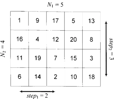
Changing the folding steps in the Chinese Remainder Theorem
The Chinese remainder theorem dictates positioning the coefficients diagonally, moving one step left and one step down. But, the autocorrelation properties can be retained even with different folding steps. In this case the positions of the coefficients are set by the equations:
ni = (n + (n - 1) • (step! - 1)) mod A/x
1.9 n2 = (n + (n - 1) • (step2 - 1)) mod N2
where step\ and stepi are the folding steps. In order for positions not to coincide the steps must not be divisor of the respective dimension. For instance, if a 20 coefficient long sequence must be folded in a 4x5 array the value of 2 can't be used for slepi. If this value is used then equation 1.9 will give n2 — (2ri)mod 4+1. This means that ni takes up only odd value which cannot be accepted since the lines 2 and 4 of the array will be empty while the locations of lines 1 and 3 will correspond to two coefficients.
appealing or even take advantage of the diffusers inner symmetries (as will be shown in Section 4.4.2).
=5
1
16
11
6
9
4
19
14
17
12
7
2
5
20
15
10
13
8
3
18
C-3
LtJ
step\ =
2
Figure 1-5. The positions of the coefficients of a 20-coefficient long sequence when folded in a 4x5 array with step\ = 2 and stepi = 3.
1.3.
Summary
[image:33.554.161.395.117.320.2]Chapter 2.
Assessing a diffuser
hi order for the quality of a diffusing structure to be established there is need for the scattered pressure distribution to be attained. In this Chapter numerical methods for the prediction of the scattered pressure of a surface will be discussed, while the measuring method that was used in this thesis will be presented.
2.1.
Prediction methods
When Schroeder introduced the concept of using phase grating to achieve sound diffusion he suggested that the far field polar pattern would be given by the Fourier transform of the reflection coefficients of the surface[8]. If a structure that displays variation of its reflection coefficient in one dimension was sampled every w and /?„ was the reflection coefficient of each sample then the far field scattered pressure would be:
N-l
f\« G 2,. L
n=0
where 9 is the angle of reflection, n is the sample number, k the wavenumber and TV the number of samples. Note that this is a Discrete Fourier Transform of kwsinO, and for this reason the prediction method is often referred to as a Fourier model.
Since then a number of methods for the prediction of the scattered pressure distribution from a surface have been developed[l 1].
2./. 1. Boundary Element Modelling (BEM)
This method uses the Helmholtz-Kirchhoff integral equation to estimate the pressure at a given point by adding the pressure direct from the source with the sum of the pressure reflected from different patches of the surface. The reflected pressure is estimated by the surface integral of the pressure and its derivative over the reflecting surface[29]:
f E E
f E S
f E D
surface s and the source of the wave respectively. p(f), Pl (f,f0 ) and p(fs ) are the pressures at the point of interest, the direct radiated pressure of the source to the receiver and that at a point on the surface, n is the normal to the surface pointing outwards, ds is an infinitely small portion of the surface and G(f,fs ) is the free field Green's function:
C(r,fs ) = where r = If — For a 2-D case Green's function is given by the Hankel function:
2.3
2.4
Where H^ is the Hankel function of the 2nd kind of order 0.
In the case that the surfaces are considered locally-reacting the pressure derivative can be connected with the pressure using the surface admittance:
2.5
where /? is the surface admittance pointing outwards from the surface. In the case of a reflective surface /?—*•() and consequently the pressure derivative can be omitted from equation 2.2.
source
point on surface s
[image:35.554.73.475.483.696.2]D
For the numerical calculation the surface must be meshed into N small elements (Figure 2-2). Their size is set usually much smaller than the wavelength so that the pressure and its derivative can be considered constant[12]. In this thesis this limit is set to a tenth of the wavelength (/1/10). The solution is then carried out in two steps. First the surface pressures on the elements are estimated and after that the pressure at any point in space can be calculated.
Figure 2-2. A plane surface meshed for a BEM.
In order for the surface pressures to be estimated eq. 2.2 must be solved simultaneously for the N surface elements. The simulation rests on solving the system of TV equations that is
shown here in the form of a matrix:
2.6
where 1N is the (N x N) identity matrix, P and P, are (1 x N) matrices of the surface pressures and the pressure directly from the source to the surface respectively and A is the (N x N)
matrix which states the contribution from the m'h element to the n" and sm is the surface of the mth element. Its coefficients are formed by introducing eq. 2.5 in the integral of eq. 2.2:
The solution of equation 2.6 can be reached by calculating the inverse of the matrix (-1N +
AJ. As a result of that the surface pressures can be estimated:
p. 2.8
Once the surface pressures are known the integral equation, forf 6 E, gives the pressure at any point in the E domain.
This method offers a direct solution to the Boundary Integral Equation and is used in the Part 2 of the thesis for the prediction of the scattered pressure distribution of Absorption Grating Diffusers[30].
Thin panel Boundary Element Modelling
In order to reduce the computation time of the method other formulation must be used. Terai[31] presented equations that connect the surface of the two sides of an infinitely thin surface which are used to form the thin panel BEM. The pressure difference p(rs i) — p(fs 2 ) between the front and back of the plate is given by the equation[31]:
n dpi(r0 ,rs<1 ) ff /- \ (~ \\ ac2 (f'^,i)
0= . V ^ +
lP(rs,i)-p(rs,2))T-———TT-dn(rs,i) i dn(rJdn(rSii 2.9
With the pressure difference known the pressure at a given external point is given by the equation:
f f ^ \ f^ M c'Hr' rsi i(r) = PiCro.rJ + J {p(rs>1 ) - p(rSi2 )} d ,f '
p.(r) = w.-irn.r, ) -t- I itMrv-i i — ZM/C? ir——7-—r~ris 2.10
Thin panel BEM ..
(a) (b)
Figure 2-3. Quadratic Residue Diffuser (QRD) geometry in the thin panel BEM.
The diffusers are attached on walls so the area of interest is the space on the front of the structure. This means that the structure can be meshed as is presented in Figure 2-3(b) since the back has very little interference with the scattering at the front of the diffuser in the higher frequency bandwidths where scattering is significant. Leaving the back open has the added advantage that there is no enclosure created that can produce non-unique solutions. This indirect solution to the Boundary Integral Equation is the ideal BEM formulation to simulate the performance of PGDs[32-33] and therefore it is used in Chapters 3 and 4[34].
When a large surface is to be modelled the Boundary Element Method can become very computationally expensive. The process can be sped up by making a number of approximations.
2.1.2. Fraunhofer or Fourier Model
The Fraunhofer Model starts from the same integral equation as the Boundary Element Method (eq. 2.2). The approximations that have been taken suggest that this model should only be considered in the far field. Consider normal incidence sound. The scattered pressure at a point in space is given by[l 1]:
jkb
8/r 2 rr
(-)
V r /
/
2.11In this equation the integration is the Fourier transform of the reflection coefficient in the
kxs sind domain. This is a similar result to the one that Schroeder reached. It is common for the (cos9 + 1) factor to be neglected and to follow the Fourier approach (eq. 2.1).
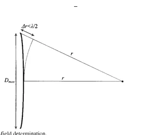
Far-Field
The far field is defined as the distance at which the difference between the minimum and the maximum path length from the panel to the receiver is small compared to the wavelength (Figure 2-4)[ll]. This region is located where the distance between the receiver and the surface is large compared to the maximum dimension of the surface:
2.12
[image:39.554.129.432.205.482.2]Dn
Figure 2-4. Far-field determination.
The first requirement is rarely an issue if the second one is met. When they are met all the point on the surface can be considered to be the same distance from the receiver[35]. The surface is in the far field when[l 1, 23, 35]:
2.13
The region that falls under the far-field category changes for oblique positions. The furthest case for small surfaces is when the receiver is in the normal of the surface. If the surface is wide, then the receivers must be further away for grazing angles.
2.2.
Scattered pressure distribution measurement methods
The measurement of the scattered pressure distribution is in the process of being internationally standardized ISO:17497-2[23]. The standard is at the moment a committee draft based on the Audio Engineering Society standard AES-4id-2001[22] and it considers measurement in a three or a two dimensional domain under free field conditions.
The simplest way of measuring polar plots is if the diffuser is 1-D. Such diffusers scatter sound in one plane and the polar response of interest is limited to two dimensions. For this measurement a semi-anechoic chamber is used[22]. The reflective floor of the chamber is taken into account by considering the image of the sample (Figure 2-5).
sample sample
D
mic
—*— source 2D mic source
Figure 2-5. Free-field equivalent of the semi-anechoic chamber.
The setup of the measurement is depicted in Figure 2-6 with the speaker being at the bottom of the figure. 37 microphones are set in an arc spaced apart by A<p-5° with a radius of R =
1.4m. The radius was dictated by the width of the room which is 3.3m. The samples that were tested had a maximum width of 10cm and a height of 30cm. If the mirror image of the samples is taken into account then they appear to be 60cm tall.
The measurements were carried out in the semi-anechoic chamber of the University of Salford. For the recording a 44 channel NetdB real-time analyzer was used (Pro-121 and Pro- 132 combined)[36-37]. The source needed to be as close to the floor of the chamber as possible (see Figure 2-5) so the Visaton SC 4 ND[38] speaker was used which has a flat response from \kHz up to 22kHz and is 5cm in diameter which resulted in its centre being 2.5cm from the floor. Since the microphones are in the path of the loudspeaker they needed to be as small as possible so as not to interfere. So they were made less than 5mm in diameter using miniature omni-directional capsules that have flat response in the range of operation of
Although far-field measurements are the ideal case for diffusion measurement they are not realistic for high frequencies (eq. 2.13) as they require a very big anechoic chamber unless the sample is really small. So the international standard requirement of 80% of the receivers being outside the specular reflection zone was met. This led the source to be placed at a distance of 3.7m for the 70cm wide samples and 3.2m for the 40cm ones. The measurements were carried out only for normal incidence due to geometric restrictions of the room.
Figure 2-6. Single plane polar response measurement set-up in the semi-anechoic chamber.
In order for the scattered impulse response of the sample to be estimated the impulse response of the sample must be de-convolved with the loudspeaker-microphone response at each scattering angle. Furthermore, the interference of the room needs to be accounted for as well. The de-convolved sample response /? is given by the equation[23]:
2.14
where FT and I FT are the forward and inverse Fourier transforms respectively. hs and hb are the impulse response with and without the sample respectively and h,.m is the loudspeaker- microphone response.
The impulse responses are measured using a Maximum Length Sequence. First the microphone-loudspeaker response h\.m is measured by positioning the loudspeaker in the place of the sample facing each microphone. Then the loudspeaker is placed facing the sample-area and two measurements are carried out one with hs and one without the sample hb
w
\i.e.
0.1
-0.1
-0.2 C
0.2
0.1
0
-0.1
.n 9
——
) 0.005
-L
i
0.01 0.015 0.02 O.C
IT
25
0.005 0.01 0.015
[image:42.554.115.433.426.687.2]time
0.02Figure 2-7. Measured impulse responces with and without the sample.
0.025
02
0.1
-0.1
-0.2 i—————i
0 0.001 0002 0.003 0004 0005 0006 0.007 0.008 0.009 0.01
time
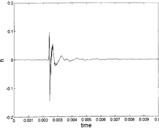
The common peak corresponds to the incident wave that gets recorded by the microphone before it reaches the sample area. The second peak of hs contains the scattered response from the sample. After the application of equation 2.14 the response is windowed to remove the residue from the incident sound. Thus the scattered impulse response that is used to generate the polar response of the sample is acquired (Figure 2-8). The polar plot for each frequency is obtained by Fourier Transforming the impulse responses of the 37 miniature microphones (Figure 2-9).
Despite the efforts to follow the standard to the letter the requirement for signal to noise ratio was not met. The standard suggests a value of at least 40dB for a reference flat plate. In the measurements carried out for this thesis the signal to noise ratio did not exceed 25dB due to the low sensitivity of the microphones used. Despite this deviation the measured scattered pressure distribution displayed the expected behaviour.
Since the sample is a flat reflective surface the scattered pressure distribution is expected to be symmetric. As can be seen in Figure 2-9 there is a notable difference for instance at ±5^/8. The reason for this is the fact that the plot suffers from errors in the positioning of the microphones in the arc. Due to the existence of sharp variations in the plot even a 0.1° error in the position of the microphone can result in a substantial error in measurement.
-71/8
-37I/: 371/8
Figure 2-9. Measured normal incidence scattered pressure distribution of a rigid surface 10cm
wide at I MHz.
2.3.
Measurements Vs Simulations
The measured sample is a Hat rigid plate of 70cm width, 10cm depth and 30cm height. Since the system discussed in the previous Section measures the scattered field in one plane 2-D simulation is going to be used for the investigation. The simulation will consider an infinitely tall surface but the measured sample is tall enough for that not to be a factor given that the area of interest is that close to the floor of the chamber.
2.3.7. Boundary Element Modelling
The geometry of the measurement is introduced in 2-D BEM and Figure 2-10 displays the polar plots of the scattered field at a number of distinct frequencies. Although the patterns are not dissimilar the reflected pressure predicted by BEM diminishes as the frequency increases. This is due the fact that the 2-D BEM considers cylindrical wave propagation which is given by a 0' order Hankel function (eq 2.4) that attenuates the sound wave with distance r as a function of r
-Ji/8 IS? 7i/8
-71/4 X
-37I/8/
-71/8 100 n/8
-71/2
-71/4 ,- '
3K/8 -37t/8/
7t/2 -71/2
3n/8 -371/1
-71/2
Figure 2-10. Normal incidence scattered pressure distribution (dB) measurement Vs BEM prediction from a rigid surface, (a) \kHz, (b) 2kHz, (c) 4kHz and (d) 6kHz. ——— Measured,
——— Predicted.
In order to compensate for this effect, the reflected pressures must be normalised to a reference pressure. In order for the reference pressure to be representative of the distance the sound wave travels the reference point can be the scattered pressure at the 0° receiver. In this way reflected energy will be lost so the normalisation will be done to the same overall reflected energy per frequency. This allows for the patterns of the scattered pressure
-71/8
-71/2
3;t/8
71/2 -71/2
-3n/i
II/2 -71/2
-3n/i
Tt/2 -Ti/2 -71/4
-71/4, -71/8
-7t/8
371/8
^ Tt/2
12? n/8
371/8
Figure 2-11. Normal incidence scattered pressure distribution (dB) measurement Vs BEM prediction from a rigid surface normalized to the same sum of the reflected pressure, (a)
IkHz, (b) 2kHz, (c) 3kHz, (d) 4kHz, (e) 5)k//c and (f) 6W/z. ——— Measured, ——— Predicted.
BEM simulation manages to predict quite accurately the distribution at small angles of reflection (< ±7r/4) while seemingly failing only at oblique angles of reflection at high frequencies. The reason for this difference is the existence of a large number of narrow periodicity lodes at high frequencies that occur so close together that they fall within the error of placing the microphones in their arc as discussed in Section 2.2.
Comparison of measurements and simulations from partly absorbing surfaces will be conducted in Section 9.2.1 where the performance of Absorption Grating Diffusers is going
to be investigated.
2.3.2. Fourier Model
[image:45.554.66.500.66.378.2]Figure 2-12 displays the polar plots of the scattered field at a number of distinct frequencies as predicted by the Fourier Model compared to measurement. Given the fact that the model does not consider wave attenuation the graphs have been normalised to the same sum of reflected pressure. At I kHz the prediction is in agreement to the measurement with the exception of the oblique angles of reflection, at 2kHz the agreement occurs only in the locations and width of the lobes while at higher frequencies there is no agreement.
-Tt/4
-371/8/
-71/2 J 71/2
-71/2
-n/4/ //T8^ "~N.1t/4
J 71/2
Figure 2-12. Normal incidence scattered pressure distribution (dB) measurement Vs the Fourier Model prediction from a rigid surface normalized to the same sum of the reflected pressure, (a) IkHz, (b) 2kHz, (c) 3kHz, (d) 4kHz, (e) 5kHz and (f) 6kHz. ——— Measured,
——— Predicted.
[image:46.554.62.505.198.511.2]can show only the potential of a structure to diffuse and not be used to access its performance.
2.3.3. Discussion
There is a trade-off between accuracy of prediction and computational speed with the different models. The Fourier Model is very fast but it is an idealization of the problem. It does not correctly model evanescent waves close to the surface, it considers incident plane waves and is only applicable in the far field. However, it is an elegant model that connects the distribution of the reflection coefficient on the surface with the scattered response. That is why it finds application in diffuser design.
The Boundary Element Method is more accurate and has been shown to give accurate predictions for Phase Grating Diffusers[31] but is computationally expensive. There are methods that allow for the number of elements to be reduced such as the thin-panel Boundary Element Method[31] or exploitation of the symmetries of the surface[ll] but even then it remains time consuming.
The angular resolution of the polar plots in this chapter have been dictated by the measurement procedure were the receivers were placed with an increment of 5°. At later stages of this thesis angular resolution of 1° will be used when predicting the performance of diffusers. This will give a better representation of the performance of diffusers.
2.4.
Summary
This Chapter contained the various methods that have been use in the past to attain the scattered pressure distribution from a diffuser. Boundary Element Modelling has been shown as the most exact but at the same time more computationally expensive simulation technique. The Fourier Model on the other hand has been shown to give a very elegant connection between the distribution of reflection coefficients on a surface and the scattered pressure distribution from it. Finally, the method to measure the scattered field that was used in this thesis has been presented and compared with both 2-D BEM and Fourier Model. In the two following Chapters PGDs are going to be discussed. In Chapter 3 the reasoning behind standard PGDs is going to be presented and issues surrounding diffuser design such as periodicity and modulation are going to be addressed. Later, in Chapter 4 new PGDs are
Chapter 3.
Diffusers
Standard
Phase
Grating
The most common category of diffusers is Phase Grating Diffusers (PGD). In this Chapter these structures are going to be presented. Their inherent limitations are going to be discussed and the issue of periodicity is going to be addressed. Modulation techniques are going to be used to be deal with the problem of periodicity.
3.1.
The diffusers
The introduction to this thesis presented sequences for PGDs, here the diffuser design is examined in more detail.
Figure 3-1. One period of a Maximum Length Sequence Diffuser (MLSD) of well width vr
r/i
and depth of the n well, dn .
Figure 3-2. One period of a Quadratic Residue Diffuser (QRD) of well width u- and depth of
th
the nm well, dn .
The depth of the «th well dn in the diffuser is set using a pseudorandom sequence[8]: