Spline Collocation Method for solving Burgers equation in Fluid Dynamic

(1)

International Journal of Emerging Technology and Advanced Engineering

Website: www.ijetae.com (ISSN 2250-2459, ISO 9001:2008 Certified Journal, Volume 7, Issue 9, September 2017)

185

Spline Collocation Method for solving Burgers equation in

Fluid Dynamic

Nileshkumar A. Patel

1

, Dr. Jigisha U.Pandya

2

1_{Department of Mathematics, Shankersinh Vaghela Bapu Institute of Technology, Gandhinagar, Gujarat, India} 2_{Department of Mathematics, Sarvajanik College of Engineering & Technology, Surat, Gujarat, India}

Abstract— In this paper, Spline collocation method is

employed to approximate the solution of Burgers equation, which is a one-dimensional non-linear partial differential equation in fluid dynamics. Our aim is to check the efficiency of the Spline Collocation Method to nonlinear partial differential equation. The Implicit and explicit solutions obtained are compared with the exact solutions. The results revel that the spline Collocation method is very effective, convenient and quite accurate to systems of partial differential equations. It can be predicted that the spline collocation method can be an efficient tool in engineering.

Keywords—Burgers equations, Spline Explicit scheme,

Spline Implicit scheme, Fluid dynamics.

I. INTRODUCTION

One of the major challenges in the field of complex systems is a thorough understanding of the phenomenon of turbulence. Direct numerical simulations have substantially contributed to our understanding of the disordered flow phenomena inevitably arising at high Reynolds numbers. However a successful theory of turbulence is still lacking which would allow predicting features of technologically important phenomena like turbulent mixing, turbulent convection, and turbulent lent combustion on the basis of the fundamental fluid dynamical equations. This is due to the fact that already the evolution equation for the simplest fluids, which are the so-called Newtonian incompressible fluids, have to take into account nonlinear as well as nonlocal properties.

( , )

( , ).

( , )

( , )...(A)

u x t

t

p x t

v u x t









 

 

In 1939 the Dutch scientist J.M.Burgers simplified the Navier-Stokes equation (A) by just dropping the pressure term. This equation can be investigated in one spatial dimension is known as Burgers equations.

Burgers model of turbulence is a very important fluid dynamics model and the study of this model and the theory of shock waves have been considered by many authors, both for conceptual understaning of a class of physical flows and for testing various numerical method. That equation (1) is the simplest mathematical formulation of the competition between nonlinear advection and viscous diffusion. It containts the simplest form of non-linear advection term u, ux and dissipation term ɛuxx where ɛ=1/Re( ɛ: kinematic viscosity and Re: Reynolds numbers) for simulating the physical phenomena of wave motion and thus determines the behaviour of the solutions. The mathematical properties of equation (1) have been studied by coles(1951). He also gave an exact solution of Burger equation. Benton and Platzman(1972) have demonstrated about 35 distinct exact solutions of Burgers-like equations and their classification.It is well known that the exact solution of Burger equation can only be computed for restricted values of ɛ which represent kinematics viscosity ofthe fluid motion. Because of this fact, various numerical methods were employed to obtain the solution of Burger’s equation with small ɛ value.

Many numerical solutions for equation (1) have been adopted over the years. Finite element technique have been employed frequently. For example Ozis et al.(2003) applied a simple finite element approach with linear elements to

Burgers equation reduced by Hopf-Cole transformation. In the case where the kinematic viscosity is small enough i.e. ɛ =0.0001, the exact solution is not available and a discrepancy exists in the literature.Also it is demonstreated that the parabolic structure of the equation decayedd for t = 0.5.In this study,the reduced Burgers equation is solved by spline explicit scheme and implicit scheme.

II. BURGER’S EQUATION

In equation (1) let us consider the following initial and boundary condition

u(x,0) = sin x in [0,1]

u(0,t) = u(1,t) = 0 , t ≥ 0

2 2

u(x,t)+u(x,t) u(x,t)= u(x,t)...(1)

t x  x

  

(2)

International Journal of Emerging Technology and Advanced Engineering

186

So first I am converting this non linear equation to in linear form using cole hofp transformation we consider

u = ψx

So that the equation (1) becomes

ψxt + ψxψxx = ɛ ψxxx

And after integration with respect to x, the equation (1) becomes

ψt + (1/2)ψx2= ɛ ψxx

If ψ = -2ɛlnϕ

Then yields øt = ɛøxx…… (2)

With the following initial and boundary conditions

 

0 = sinπ in [0,1]

0,t =

1,t = 0 ,

x

t

,

0 x





Now discritizing left side equation(2) by forward difference formula and replacing right side by the second derivatives Sˈˈ(xi) at jth level like explicit scheme in finite

difference,we get

i-1, j 1 i, j 1 i+1, j 1

i-1, j i, j i+1, j

...(6) 2

where r = t/h 4

= (1+6r) (4 - 12r) (1 6r)

               

Equation(6) is known as Spline Explicit formula.

Same as we discretizing left side of equation(2) by forward difference formula and replacing right side by the second derivatives Sˈˈ(xi) at jth and j+1th level like explicit

scheme in finite difference, we get

Equation(11) is known as Spline Explicit formula.

III. EXPLICIT SOLUTION

In equation (6) we consider ɛ =1 and ∆t = 0,001 and h = 0.1, then we get

1+ (6∆t/h2) = 1.6 & 4-(12∆t/h2) = 2.8 If j = 0 and i =1 to 9 consider then we get

0,1 1,1 2,1

1,1 2,1 3,1

2,1 3,1 4,1

4 1.80570

4 3.434653

4 4.727394















'' i, j 1 i, j i,j

'' '' th

i,j i

'' i,j '' '' '' 2 i-1,j i,j i-1,j i-1

( - ) / t S ...(3) where S denote S (x ) at j level

substitute values of S in the below equation

S 4S +S (6/h )(

  



  

  _,j _{i, j} _{i 1, j})

( _{i-1, j 1} - _{i-1, j}) (_{i, j 1} - _{i, j}) (_{i+1, j 1} - _{i+1, j}) 4

t t t

6

₂ _i-1,j - 2 _{i, j} + _{i 1, j} ... h

- 2 + ...(4) then we get

             _        

 _ _ _ ..(5)

i, j 1 i, j '' '' i,j i,j+1 '' ''

i,j i,j+1 i

i-1, j i, j i 1, j

i 2

-

(S S ) ...(7)

t 2

where S , S denote second derivatives

at x = x the time level j and j+1 respectively.

S S S

6 ( h   



          

-1,j i, j i 1, j i-1, j 1 i, j 1 i 1, j 1

i-1,j 1 i, j 1 i 1, j 1 2

- 2 + ) ...(8)

S S S

6

( - 2 + ) ...(9)

h                     2

(2 / t) ( _{i-1, j 1}- _{i-1, j}) - S_{i-1, j}

4 (2 / t) (_{i, j 1}- _{i, j}) - S_{i, j}

(2 / t) ( _{i 1, j 1} - _{i 1, j}) S_{i 1, j}

(6/h ) ( _{i-1, j 1} - 2 _{i, j 1} _{i 1, j 1}) ...(10)

(1 3 which gives r               _     _    _ _ _  _  _ _  _ _ 









)_{i-1, j 1} (4 6 )_{i, j 1} (1 3 ) _{i-1, j 1}

(1 3 ) _{i-1, j} (4 6 )_{i, j} (1 3 ) _{i-1, j}. ...(11)

r r

r r r

  

   

  

(3)

International Journal of Emerging Technology and Advanced Engineering

187

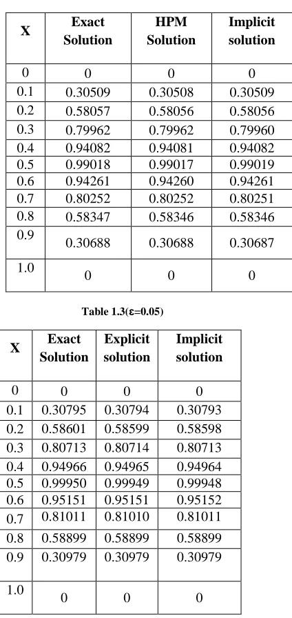
Solving above system of nine equations in nine unknowns with the help of Matlab, we get the solution as shown in table below (1.1) and these solutions are compared with the exact solutions.

IV. IMPLICIT SOLUTION

In equation (11) we consider ɛ =1 and ∆t = 0.001 and h = 0.1, then we get

1-(3∆t/h2) = 0.7, 1+ (3∆t/h2) = 1.3 4+ (6∆t/h2) = 4.6, 4-(6∆t/h2) = 3.4

In equation (11) we consider j=0 and i=1 to 9 then we get

V. EXPLICIT SOLUTION

In equation (6) we consider ɛ =0.05 and ∆t = 0.001 and h = 0.1, then we get

1+ (6ɛ∆t/h2) = 1.03 & 4-(12ɛ∆t/h2) = 3.94

In equation (6) we consider j=0 and i=1 to 9 then we get

VI. IMPLICIT SOLUTION

In equation (11) we consider ɛ =0.05 and ∆t = 0.001 and h = 0.1, then we get

1-(3ɛ∆t/h2) =0.985, 1+ (3ɛ∆t/h2) = 1.015 4+ (6ɛ∆t/h2) = 4.03, 4 - (6ɛ∆t/h2) = 3.97

3,1 4,1 5,1

4,1 5,1 6,1

5,1 6,1 7,1

6,1 7,1 8,1

7,1 8,1 9,1

8,1 9,1 10,1

4 5.557385

4 5.843380

4 5.557385

4 4.727394

4 3.434653

4 1.805703



























0,1 1,1 2,1

1,1 2,1 3,1

2,1 3,1 4,1

(0.7) (4.6) (0.7) 1.814778

(0.7) (4.6) (0.7) 3.451914

(0.7) (4.6) (0.7) 4.751152

  

  

3,1 4,1 5,1

4,1 5,1 6,1

5,1 6,1 7,1

6,1 7,1 8,1

7,1 8,1 9,1

(0.7) (4.6) (0.7) 5,585314

(0.7) (4.6) (0.7) 5.872746

(0.7) (4.6) (0.7) 5.585314

(0.7) (4.6) (0.7) 4.751152

(0.7) (4.6) (0.7) 3.451914

(0.7)

  

  

8,1 (4.6) 9,1 (0.7) 10,1 1.814778

     

0,1 1,1 2,1

1,1 2,1 3,1

2,1 3,1 4,1

4 1.822945

4 3.467448

4 4.772533

  

  

3,1 4,1 5,1

4,1 5,1 6,1

5,1 6,1 7,1

6,1 7,1 8,1

7,1 8,1 9,1

8,1 9,1 10,1

4 5.610450

4 5.899176

4 5.610450

4 4.772533

4 3.467448

4 1.822945

  

  

(4)

International Journal of Emerging Technology and Advanced Engineering

188

In equation (11) we consider j = 0 and i =1 to 9 then we get

VII. TABLES

Table 1.1 (ɛ=1)

Table 1.2(ɛ=1)

Table 1.3(ɛ=0.05)

X Exact

Solution

HPM Solution

Explicit solution

0 0 0 0

0.1 0.30509 0.30508 0.30510

0.2 0.58057 0.58056 0.58055

0.3 0.79962 0.79962 0.79961

0.4 0.94082 0.94081 0.94081

0.5 0.99018 0.99017 0.99017

0.6 0.94261 0.94260 0.94258

0.7 0.80252 0.80252 0.80250

0.8 0.58347 0.58346 0.58345

0.9 0.30688 0.30688 0.30687

1.0 0 0 0

X Exact

Solution

HPM Solution

Implicit solution

0 0 0 0

0.1 0.30509 0.30508 0.30509

0.2 0.58057 0.58056 0.58056

0.3 0.79962 0.79962 0.79960

0.4 0.94082 0.94081 0.94082

0.5 0.99018 0.99017 0.99019

0.6 0.94261 0.94260 0.94261

0.7 0.80252 0.80252 0.80251

0.8 0.58347 0.58346 0.58346

0.9

0.30688 0.30688 0.30687

1.0

0 0 0

X Exact

Solution

Explicit solution

Implicit solution

0 0 0 0

0.1 0.30795 0.30794 0.30793 0.2 0.58601 0.58599 0.58598 0.3 0.80713 0.80714 0.80713 0.4 0.94966 0.94965 0.94964 0.5 0.99950 0.99949 0.99948 0.6 0.95151 0.95151 0.95152 0.7 0.81011 0.81010 0.81011 0.8 0.58899 0.58899 0.58899 0.9 0.30979 0.30979 0.30979

1.0

0 0 0

0,1 1,1 2,1

1,1 2,1 3,1

2,1 3,1 4,1

3,1 4,1 5,1

(0.985) (4.03) (0.985) = 1.823399

(0.985) (4.03) (0.985) 3.473531

(0.985) (4.03) (0.985) 4.773721

(0.985) (4.03) (0.985) 5.611846

  

 

  

4,1 5,1 6,1 5,1 6,1 7,1 6,1 7,1 8,1 7,1 8,1 9,1 8,1 9,1

(0.985) (4.03) (0.985) 5.900644

(0.985) (4.03) (0.985) 5.611846

(0.985) (4.03) (0.985) 4.773721

(0.985) (4.03) (0.985) 3.473531

(0.985) (4.03)

  

 

  

[image:4.612.355.567.150.598.2] [image:4.612.61.255.432.673.2]

(5)

International Journal of Emerging Technology and Advanced Engineering

189

VIII. GRAPHICAL

Graph 2.1(Explicit) ɛ=1

Graph 2.2(Implicit) ɛ=1

IX. CONCLUSION

In this study, the spline explicit and implicit scheme method has been successfully applied to the Burger’s equation with specified initial conditions.

The results showed that these method are powerful mathematical tools for solving Burgers equation and very effective, convenient and quite accurate to systems of Partial differential equations.

REFERENCES

[1] Noorzad, Reza, A. Tahmasebi Poor, and Mehdi Omidvar. "Variational iteration method and homotopy-perturbation method for solving Burgers equation in fluid dynamics." Journal of Applied Sciences 8.2 (2008): 369-373.

[2] Blue, James L. “Spline Function Methods for Nonlinear Value Problems.” Spline Function Methods for Nonlinear Boundary-Value Problems, vol. 12, Magazine Communications of the ACM, 1969, pp. 327–330.

[3] Gorguis, Alice. "A comparison between Cole–Hopf transformation and the decomposition method for solving Burgers’ equations." Applied Mathematics and Computation 173.1 (2006): 126-136. [4] Kleinmichel, H. "JH Ahlberg, EN Nilson, JL Walsh, The Theory of

Splines and Their Applications.(Mathematics in Science and Engineering, Volume 38.) Academic Press." ZAMM‐Journal of Applied Mathematics and Mechanics 50.6 (1970): 441-442. [5] Sachdev, P. L. "A generalised Cole-Hopf transformation for

nonlinear parabolic and hyperbolic equations."Mathematics and Physics (ZAMP) 29.6 (1978): 963-970.

[6] Doctor H. D., Bulsari A. B. and Kalthia N. L.: “Spline collocation approach to boundary value problems”, Vol. 4, No. 6(1984):511-517.