Position Control for Electromagnetic Suspension System using FLC

(1)

International Journal of Emerging Technology and Advanced Engineering

Website: www.ijetae.com (ISSN 2250-2459,ISO 9001:2008 Certified Journal, Volume 4, Issue 6, June 2014)

329

Position Control for Electromagnetic Suspension System

using FLC

Ashwani Soni

1

, Abhishek Garg

2

, Nikhil Kumar

3

, Nitin Kumar

4

, Akanksha Tayal

5 , Anurag Singhal6 1,2,3,4,5

Lecturer, Shobhit University, Gangoh

6_{Student, Shobhit University, Meerut}

Abstract--Magnetic levitation refers to suspending an object in air without any physical support, just using magnetic force to counter balance weight of the object and any other force acting on the object. If magnetic attraction

is used it is called magnetic suspension and if magnetic

repulsion is used the phenomenon is called magnetic

levitation.

This paper presents PID, Fuzzy Logic Controller for an Electromagnetic Suspension System (EMS) system which is a nonlinear system. In this paper we consider the tracking control problems for an electromagnetic levitation system by using Jacobi Linearization Technique. We first derive a nonlinear state equation of the electromagnetic levitation system. We then design tracking controllers using the PID and FLC. For the tracking control a unit step trajectory is taken as the reference signal.

The simulation result shows that Fuzzy Logic Controller has better control performance as compare to PID controller for Electromagnetic Suspension (EMS) System.

Keywords--- Fuzzy Logic control, Proportional–Integral– Derivative (PID), EMS, Jacobi Linearization Technique, Ziegler-Nichols Tuning method.

I. INTRODUCTION

The Electromagnetic Suspension System (EMS) system is composed of an LED light source, an electromagnet, an optoelectronic sensor, amplifier module, an analogue control module, data acquisition card, and a steel ball, etc. Its structure is simple, yet the control effect is very intuitionist and interesting. EMS system works via the force of attraction between an electromagnet and the object [1]. If the object gets too close to the electromagnet, the current in the electromagnet must be reduced. If the object gets too far, the current in the electromagnet must be increased to pull back the object to the equilibrium point. It is a nonlinear, third order, open loop unstable system [2].

II. MODELLING OF THE PLANT

The main challenge in controlling the position of the suspended object is to maintain the balance of the weight of the suspended object and the electromagnetic force acting on it. In this paper we are interested only in

controlling the vertical position of the suspended object.

Thus all the dynamics will be concerned to vertical motion of the suspended object [3].

Figure1: Electromagnetic Levitation Experiment System Configuration

The dynamics of the electromagnet is given by-

Where,

= the source voltage

= series resistance of the circuit i = current flowing in the electromagnet

= inductance when ball is not present.

= inductance when ball is next to the coil.

= constant [4].

(2)

International Journal of Emerging Technology and Advanced Engineering

330

Where,

= mass of the suspended object

= acceleration due to gravity

= distance of ball surface from the bottom of the

electromagnet

= coefficient of viscous friction

= current in the coil

= force generated by the electromagnet

Now energy stored in the electromagnet is given as

Thus, the force is calculated as

Using above expression of , the differential

equation governing the motion of the suspended object is given as

Defining the state variables as

(Position),

(Velocity),

(Current)

Control input as and

Output as

The state model is given as:

Above nonlinear state model can be written as

Where,

III. LINEARIZATION AND TRANSFER FUNCTION

The nonlinear dynamics of the system are linearized about the equilibrium point by Jacobi linearization [5] and the linearized system is obtained as below:

(3)

International Journal of Emerging Technology and Advanced Engineering

331

Where,

[image:3.595.61.268.221.433.2]

The parameters’ real-plant values used for simulation are given below [6]:

Table 1:

System Parameters for Simulation

Using these parameters the matrices from above expressions are –

Also transfer function of the plant is obtained as

IV. PIDCONTROLLER

PID is named after the three terms which together constitute the manipulated variables. The proportional, integral and Derivative terms are summed to result PID controller output [7]. Defining S (t) as the PID controller output the final form of PID algorithm is

S (t) = Kp e (t) + Ki ∫e (t) dt + Kd de/dt

Where Kp, Ki, Kd are proportional gain, Integral gain

and Derivative gain. The signal e(t) defined as e(t) = r(t)

−c(t) is the error signal between the reference and the

process output c(t).The Ziegler-Nichols tuning method [8] has been used to determine the controller parameters Kp, Ti, ,Td.

4.1Simulation Testing and Response:

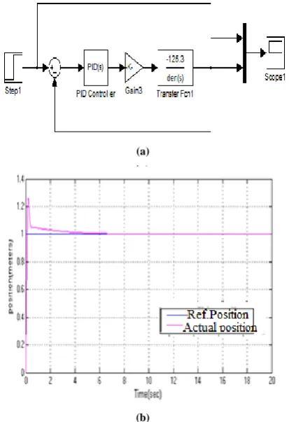
(a)

(b)

Figure 2: (a) Simulink Block Diagram and (b) Response of PID controller

4.2 For set point tracking-

Rise Time (sec) =0.4, Settling time (sec) =6.7, Overshoot (%) =27, Steady state error = 0 %

V. FUZZY LOGIC CONTROLLER

[image:3.595.329.536.247.549.2]

(4)

International Journal of Emerging Technology and Advanced Engineering

[image:4.595.64.268.139.242.2]

332

Figure 3: Block Diagram of Fuzzy Inference System

The FLC implemented here is a two-input & single-output. The two inputs are error, and error rate. Both input variables are classified into seven fuzzy levels in this implementation based on the resolution and real-time requirements needed.

[image:4.595.322.535.237.400.2]

5.1 Simulation Testing and Result

Figure 4: Simulink Block Diagram of FLC

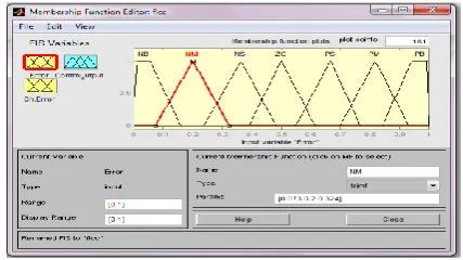
5.2 Subsets for Inputs and Output: 5.2.1 Input 1(Error):

Membership Functions for input1: NB (Negative Big), NM (Negative medium), NS (Negative small), ZO (Zero), PS (Positive Small), PM (Positive Medium), PB (Positive Big).

Figure 5: Membership function for error

5.2.2 Input 2 (Error Rate):

NB (change in error rate is Negative Big), NM (change in error rate is Negative Medium), NS (change in error rate is Negative small), ZO (change in error rate is Zero), PS (change in error rate is positive Small), PM (change in error rate is Positive Medium), PB (change in error rate is Positive Big)

[image:4.595.55.270.340.455.2]

5.2.3 Membership Functions for input 2:

Figure 6: Membership function for error rate

5.2.4 Controller Output:

Membership Functions for Output: NB (Negative Big Output), NM (Negative medium Output), NS (Negative small Output), ZO (Zero Output), PS (Positive Small Output), PM (Positive Medium Output), PB (Positive Big Output).

[image:4.595.319.544.491.657.2] [image:4.595.56.270.558.678.2]

(5)

International Journal of Emerging Technology and Advanced Engineering

333

[image:5.595.324.533.146.347.2]

5.3 Rule Base:

Figure 8: Fuzzy IF-Then Rules

5.4 Surface Viewer:

[image:5.595.52.277.148.306.2]

In this paper this plot is generated by the Forty nine rules that accounted for both error and change in error.

Figure 9: Surface Analysis of Both Inputs and Output

5.5 Rule Viewer:

This Rule Viewer provides an animation of how the rules are fired during simulation.

Figure 10: Mesh Analysis of Both Inputs and Output

[image:5.595.57.269.359.506.2]

5.6 Output response of Fuzzy Controller

Figure 11: Output response of Fuzzy Controller

5.7 For set point tracking-

Rise Time (sec) = 0.4, Settling time (sec) =0.7

Overshoot (%) =0, Steady state error (%) = 0

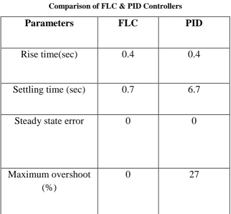
VI. RESULTS AND DISCUSSIONS

The paper presented an overview of PID controller and

FLC. PID Controller gives high overshoot and settling

time with zero steady state error. The Fuzzy Logic controller gives no overshoot, zero steady state error and smaller settling time.

Table 2

Comparison of FLC & PID Controllers

Parameters FLC PID

Rise time(sec) 0.4 0.4

Settling time (sec) 0.7 6.7

Steady state error 0 0

Maximum overshoot (%)

[image:5.595.315.548.513.729.2] [image:5.595.61.268.569.703.2]

(6)

International Journal of Emerging Technology and Advanced Engineering

334

VII. CONCLUSIONS

This paper presents a comparative study of performance of PID and FLC. Based on the results and the analysis, a conclusion has been made that that FLC

provides a better control action. Fuzzy PID control

scheme used only the PD portion with an integral term added to eliminate steady-state error.

Acknowledgements

The authors gratefully acknowledge the contributions of Amit Kumar, Brijendra Kumar Maurya, Haseena B.A. and Nikhil Pachauri for their work on the original version of this document.

REFERENCES

[1 ] Slotine J.-J.E. and Li W., Applied Nonlinear Control, New Jersey, Prentice Hall, 1991

[2 ] Khalil H.K., Nonlinear Systems, 3rd_{Ed, New Jersey, Prentice}

Hall, 2002

[3 ] Zak S. h., Systems and Control, New York, Oxford University Press, 2003

[4 ] Isidori, A., Nonlinear Control Systems, 3rd_{Ed., London, Springer,}

1995

[5 ] Gopal, M., Digital Control and State Variable Methods, 3rd Ed, New Delhi, Tata McGraw Hill Education Private Limited, 2009 [6 ] Gopal, M., Control Systems: Principles And Design, 3rd_{Ed, New}

Delhi, Tata McGraw Hill, 2008

[7 ] Ogata, K., Modern Control Engineering, 4th_{Ed., Englewood}

Cliffs, NJ, Prentice Hall, 2001

[8 ] Woodson, H.H. and Melcher, J.R., Electromechanical Dynamics, Part I: Discrete Systems, John Wiley, New York, 1968

[9 ] Hanley J.A., “Design And Implementation Of A Feedback Linearizing Controller And Kalman Filter For A Magnetic Levitation System”, M.S. Project Report, The University Of Texas At Arlington, 2007

[10 ]Barie W. and Chiasson J., “Linear And Nonlinear State-Space Controllers For Magnetic Levitation”, International Journal Of System Science, Vol. 27, No. 11, pp. 1153-1163, 1996

[11 ]Hurley W.G. and Wolfle W.H., “Electromagnetic Design Of A Magnetic Suspension System”, IEEE Transaction on Education, Vol. 40, No. 2, May 1997