Two Dimensional Electrostatic Problem in a Plane with Earthed Elliptic Cavity due to One or Two Collinear Charged Electrostatic Strips

Volume 2007, Article ID 60595,9pages doi:10.1155/2007/60595

Research Article

Two-Dimensional Electrostatic Problem in a Plane with

Earthed Elliptic Cavity due to One or Two Collinear

Charged Electrostatic Strips

B. M. Singh, J. G. Rokne, and R. S. Dhaliwal

Received 16 August 2006; Accepted 23 November 2006

Recommended by Hans Engler

A two-dimensional electrostatic problem in a plane with earthed elliptic cavity due to one or two charged electrostatic strips is considered. Using the integral transform technique, each problem is reduced to the solution of triple integral equations with sine kernels and weight functions. Closed-form solutions of the set of triple integral equations are ob-tained. Also closed-form expressions are obtained for charge density of the strips. Finally, the numerical results for the charge density are given in the form of tables.

Copyright © 2007 Hindawi Publishing Corporation. All rights reserved.

1. Introduction

γ

y

d

o c _γ

A B

a b x

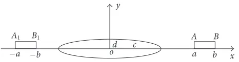
Figure 1.1. One charged strip in a plane with elliptic cavity.

y

d

o c

A B

a b x

A1 B1

a b

Figure 1.2. Two charged collinear strips in a plane with elliptic cavity.

In this paper, we consider two-dimensional electrostatic problems in a plane with an earthed elliptic cavity and (i) one charged strip of finite length aty=0,a < x < b; (ii) two charged strips of finite length aty=0,a <|x|< b. The geometry of the problems is shown in Figures1.1,1.2. Using the integral transform technique, each problem is reduced into triple integral equations with weight functions.

Closed-form solutions of the triple integral equations are obtained by using the method discussed by Singh [3,8]. In each problem, we have obtained the closed form expressions for the charge density of the strips. The numerical results are given for the charge density in the form of tables. These types of problems have application in mathe-matical physics.

As we know, an analytic solution has some advantages over numerical and approxi-mate solutions so that in many cases, analytical solutions in closed form are desired for accurate analysis and design. Moreover, analytical solutions can serve as a benchmark for the purpose of judging the accuracy and efficiency of various numerical and approximate methods.

2. Basic equations

In Cartesian coordinates (x,y), an ellipse centered at the origin is given by the equation

x2 c2 +

y2

d2 =1. (2.1)

We introduce elliptic coordinates (ξ,η), which are defined by

whereξ≥0, 0< η <2π, andl=(c2_−d2₎1/2_{. The ellipse becomes the coordinate line}

ξ=γ=cosh−1

c l

, 0< η <2π. (2.3)

In elliptic coordinates, the electrostatic potential functionV satisfies the differential equation

∂2_V ∂ξ2 +

∂2_V

∂η2 =0. (2.4)

3. Boundary conditions and solution of problem (2.1)

Due to the geometric symmetry, the problem reduces to finding a functionV(ξ,η) satis-fying (2.4) in the regionγ < ξ≤ ∞, 0≤η≤πsubject to the conditions

V(ξ,π)=0, ξ > γ,

V(γ,η)=0, 0< η < π, (3.1)

V(ξ, 0)=Δ(ξ), α < ξ < β,

∂V(ξ,η)

∂η

η=0

=0, γ < ξ < α,β < ξ, (3.2)

where

α=cosh−1

a l

, β=cosh−1

b l

. (3.3)

We can easily find the solution of Laplace equation (2.4) in the form

V(ξ,η)=

_∞

0

sinhu(π−η) sinh(uπ) f(u) sin

u(ξ−γ)du, (3.4)

which satisfies the boundary conditions (3.1) identically and the remaining conditions (3.2) lead to the following triple integral equations:

_∞

0 f(u) sin

u(ξ−γ)du=Δ(ξ), α < ξ < β,

_∞

0 ucoth(πu)f(u) sin

u(ξ−γ)du=0, γ < ξ < α,β < ξ,

(3.5)

for the determination of f(u).

On introducingx1=ξ−γ,a1=α−γ,b1=β−γ, the above equations (3.5) reduce to

the following integral equations:

_∞

0 f(u) sin

ux1 du=Δ

x1+γ , a1< x1< b1, (3.6)

_∞

Assuming

∞

0 coth(πu)u f(u) sin

ux1 du=π

2R

x1 , a1< x1< b1, (3.8)

we find its inverse Fourier sine transform as

u f(u) coth(πu)=

_b1

a1

R(t) sin(ut)dt. (3.9)

Substituting from (3.9) into (3.6), interchanging the order of integrations and using the following integral from Gradshteyn and Ryzhik (see [9, 4.117(2), page 516]):

_∞

0 u

−1_tanh(

uπ) sin(ut) sinux1 du=1

2log

sinhx1/2 + sinh(t/2)

sinhx1/2 −sinh(t/2)

, (3.10)

we find that

_b1

a1

R(t) logsinh

x1/2 + sinh(t/2)

sinhx1/2 −sinh(t/2)

dt=2Δx1+γ , a1< x1< b1. (3.11)

Differentiating both sides of the above equation with respect tox1, we find that

_b1

a1

R(t) sinh(t/2)dt

cosh(t)−coshx1 =

Δ_x1+γ coshx1/2 =p1

x1 (say), a1< x1< b1, (3.12)

where prime denotes the derivative with respect tox1. Making use of a suitable Tricomi

theorem given by Singh [3], we find that

R(t)= −2 cosh(t/2)

π2

_cosh(

t)−cosha1

coshb1 −cosh(t)

1/2

×

_b1

a1

_cosh

b1 −cosh(y)

cosh(y)−cosha1

1/2 _sinh(

y)p(y)dy

cosh(y)−cosh(t)

+ 2C1cosh(t/2)

cosh(t)−cosha1

coshb1 −cosh(t) 1/2

, a1< t < b1,

(3.13)

whereC1is an arbitrary constant. IfΔ(x1) is constant such that

Δx1+γ =Δ1(constant), (3.14)

we find that

px1 =0, (3.15)

and from (3.13), we find that

R(t)= 2C1cosh(t/2)

cosh(t)−cosha1 coshb1 −cosh(t) 1/2

Substituting the value ofR(t) from (3.16) into (3.11) and using the integral

_b1

a1

cosh(t/2) logsinhx1/2 + sinh(t/2) /

sinhx1/2 −sinh(t/2) dt

cosh(t)−cosha1 coshb1 −cosh(t) 1/2

= π

sinhb1/2 K

_sinh

a1/2

sinhb1/2

, a1< t < b1,

(3.17)

we find that

C1= Δ1

πK(δ)sinh

b1

2

, (3.18)

where

δ=sinh

a1/2

sinhb1/2

, (3.19)

andK() is the complete integral defined in Gradshteyn and Ryzhik (see [9, page 905]). From (3.16) and (3.18), we find that

R(t)= Δ1cosh(t/2) sinh

b1/2 πK(δ)cosh2(t/2)−cosh2a1/2

cosh2b1/2 −cosh2(t/2)

1/2, a1< t < b1.

(3.20)

The charge density of the strip is defined by the relation

σ1= −1

4lπsinh(ξ)

∂V(ξ,η)

∂η

η=0

= 1

4lπsinh(ξ)

_∞

0 u f(u) coth(uπ) sinh

u(ξ−γ)du, α < ξ < β,η=0.

(3.21)

The above equation can be written in the form

σ1= R

x1

8πsinh(ξ)l

= Δ1sinh

(β−γ)/2 cosh(ξ−γ)/2 8πsinh(ξ)K(δ)sinh2(ξ−γ)/2 −sinh2

a1/2

sinh2b1/2 −sinh2

(ξ−γ)/2 1/2l,

a < x < b, y=0,

(3.22)

where

ξ=cosh−1

x l

, a1=cosh−1

a l

−γ, b1=cosh−1

b l

−γ. (3.23)

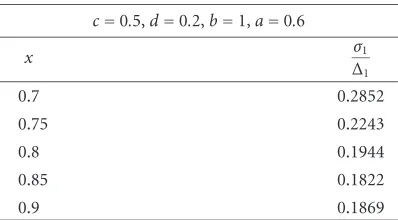
Table 3.1. Numerical results for problem (2.1).

c=0.5,d=0.2,b=1,a=0.6

x _Δσ1

1 0.7 0.2852 0.75 0.2243 0.8 0.1944 0.85 0.1822 0.9 0.1869

4. Boundary conditions and solution of problem (2.2)

Since the configuration to be investigated in problem (2.2) is symmetric with respect tox

andyaxes, we require to find an electrostatic functionV(ξ,η) which is harmonic in the regionγ < ξ <∞, 0< η < π/2 and satisfies the conditions

∂V(ξ,η)

∂η

η=π/2=

0, ξ > γ, (4.1)

V(γ,η)=0, 0< η <π

2, (4.2)

V(ξ, 0)=V0(ξ), α < ξ < β, (4.3)

∂V(ξ,η)

∂η

η=0

=0, γ < ξ < α,β < ξ. (4.4)

Suitable solution of (4.4) can be written in the form

V(ξ,η)=

_∞

0

A(u) coshu(π/2−η) cosh(πu/2) sin

(ξ−γ)udu, (4.5)

which satisfies conditions (4.1) and (4.2), and the conditions (4.3) and (4.4) give rise to the following integral equations:

_∞

0 A(u) sin

ux1 du=V0

x1+γ , a1< x1< b1, (4.6)

_∞

0 uA(u) tanh

uπ

2

sinux1 du=0, 0< x1< a1,b1< x1<∞, (4.7)

for the determination ofA(u). By assuming

∞

0 uA(u) tanh

uπ

2

sinux1 du=R0

x1 , a1< x1< b1, (4.8)

and using (4.7), we find that

uA(u) tanh

uπ

2

=2

π

_b1

a1

Substituting from (4.9) into (4.6), interchanging the order of integrations and using the following integral from Gradshteyn and Ryzhik (see [9, 4.116(3), page 516]):

_∞

0 u

−1_cothuπ

2

sin(ut) sinux1 du=1

2log

tanhx1+ tanht

tanhx1−tanht

, (4.10)

we find that

1

π

_b1

a1

R0(t)

tanhx1+ tanht

tanhx1−tanht

dt=V0

x1+γ , a1< x1< b1. (4.11)

Differentiating both sides of the above equation with respect tox1, we obtain

1

π

_b1

a1

2R0(t) tanh(t)dt

tanh2(t)−tanh2x1

=V0

x1+γ

sech2x1

=px1 (say), a1< x1< b1, (4.12)

where prime denotes the derivative with respect tox1. Using a suitable Tricomi theorem

given by Singh [3], we find that

R0(t)= −sech 2

(t)

π

_tanh2₍

t)−tanh2a1

tanh2b2 −tanh2(t)

1/2

×

_b1

a1

_tanh2

b1 −tanh2

x1

tanh2x1 −tanh2a1

1/2

2 tanhx1 sech2

x1 p

x1 dx1

tanh2x1 −tanh2(t)

+ C2sech

2

(t)

tanh2(t)−tanh2a1

tanh2b1 −tanh2(t)

1/2, a1< t < b1,

(4.13)

whereC2is an arbitrary constant. If we assume thatV0(x1+γ)=Δ0(constant), then we

find that

px1 =0, (4.14)

R0(t)= C2sech

2

(t)

tanh2(t)−tanh2a1

tanh2b1 −tanh2(t)

1/2. (4.15)

Substituting the value ofR0(t) from (4.15) into (4.11) and using the integral

_b1

a1

sech2tlogtanhx1 + tanh(t) /tanhx1 −tanh(t) dt

tanh2(t)−tanh2a1

tanh2b1 −tanh2(t) 1/2

= π

tanhb1 K

_tanh

a1

tanhb1

, a1< x1< b1,

(4.16)

we obtain

C2= Δ0tanh

b1

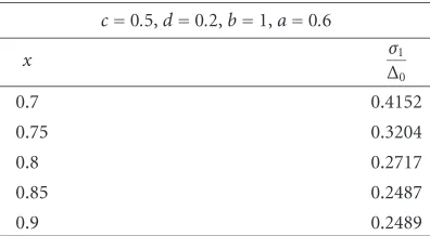
Table 4.1. Numerical results for problem (2.2).

c=0.5,d=0.2,b=1,a=0.6

x _Δσ1

0 0.7 0.4152 0.75 0.3204 0.8 0.2717 0.85 0.2487 0.9 0.2489

whereK() is the complete integral defined in Gradshteyn and Ryzhik (see [9, page 905]). From (4.15) and (4.17), we find that

R0(t)= sech

2

(t) tanhb1 Δ0 Ktanha1/tanhb1 tanh2(t)−tanh2

a1

tanh2b1 −tanh2(t) 1/2

, a < t < b.

(4.18)

The charge density is given by

σ1= −1

sinh(ξ)l

∂V(ξ,η)

∂η

η=0

= 1

sinh(ξ)l

_∞

0 A(u) tanh

πu

2

sinu(ξ−γ)du= R0

x1

4πsinh(ξ)l

= sech

2 x1 tanh

b1 Δ0

4πsinh(ξ)Kδ1 tanh2x1−tanh2a1 tanh2b1−tanh2x1

1/2, a1< x1< b1, y=0,

(4.19)

where

δ1=tanh

a1

tanhb1 . (4.20)

The above result may be written in the following form:

σ1= sech

2

(ξ−γ) tanh(β−γ)Δ0

4πsinh(ξ)Kδ1 tanh2(ξ−γ)−tanh2a1 tanh2b1−tanh2(ξ−γ) 1/2l

,

a < x < b, y=0.

(4.21)

References

[1] C. J. Tranter, “Some triple integral equations,” Proceedings of the Glasgow Mathematical

Associa-tion, vol. 4, pp. 200–203 (1960), 1960.

[2] K. N. Srivastava and M. Lowengrub, “Finite Hilbert transform technique for triple integral equa-tions with trigonometric kernels,” Proceedings of the Royal Society of Edinburgh. Section A.

Math-ematics, vol. 68, pp. 309–321, 1970.

[3] B. M. Singh, “On triple integral equations,” Glascow Mathematical Journal, vol. 14, pp. 174–178, 1973.

[4] B. M. Singh, “Quadruple trigonometrical integral equations and their application to electrostat-ics,” Journal of Mathematical and Physical Sciences, vol. 9, no. 5, pp. 459–469, 1975.

[5] B. M. Singh, J. G. Rokne, and R. S. Dhaliwal, “Quadruple trigonometrical series equations and their application to an inclusion problem in the theory of elasticity,” Studies in Applied

Mathe-matics, vol. 112, no. 1, pp. 17–37, 2004.

[6] D. A. Spence, “A Wiener-Hopf solution to the triple integral equations for the electrified disc in a coplanar gap,” Proceedings of the Cambridge Philosophical Society, vol. 68, pp. 529–545, 1970. [7] I. N. Sneddon, Mixed Boundary Value Problems in Potential Theory, North-Holland, Amsterdam,

The Netherlands, 1966.

[8] B. M. Singh, “On triple trigonometrical integral equations,” Zeitschrift f¨ur Angewandte

Mathe-matik und Mechanik, vol. 53, pp. 420–421, 1973.

[9] I. S. Gradshteyn and I. M. Ryzhik, Table of Integrals, Series, and Products, Academic Press, New York, NY, USA, 4th edition, 1965.

B. M. Singh: Department of Computer Science, The University of Calgary, Calgary, Alberta, Canada T2N-1N4

Email address:[email protected]

J. G. Rokne: Department of Computer Science, The University of Calgary, Calgary, Alberta, Canada T2N-1N4

Email address:[email protected]

R. S. Dhaliwal: Department of Mathematics and Statistics, The University of Calgary, Calgary, Alberta, Canada T2N-1N4