R E S E A R C H
Open Access
A comparison framework and guideline
of clustering methods for mass cytometry
data
Xiao Liu
1†, Weichen Song
2†, Brandon Y. Wong
1,3, Ting Zhang
1, Shunying Yu
2, Guan Ning Lin
1,2*and
Xianting Ding
1*Abstract
Background:With the expanding applications of mass cytometry in medical research, a wide variety of clustering methods, both semi-supervised and unsupervised, have been developed for data analysis. Selecting the optimal clustering method can accelerate the identification of meaningful cell populations.
Result:To address this issue, we compared three classes of performance measures,“precision”as external
evaluation,“coherence”as internal evaluation, and stability, of nine methods based on six independent benchmark datasets. Seven unsupervised methods (Accense, Xshift, PhenoGraph, FlowSOM, flowMeans, DEPECHE, and kmeans) and two semi-supervised methods (Automated Cell-type Discovery and Classification and linear discriminant analysis (LDA)) are tested on six mass cytometry datasets. We compute and compare all defined performance measures against random subsampling, varying sample sizes, and the number of clusters for each method. LDA reproduces the manual labels most precisely but does not rank top in internal evaluation. PhenoGraph and FlowSOM perform better than other unsupervised tools in precision, coherence, and stability. PhenoGraph and Xshift are more robust when detecting refined sub-clusters, whereas DEPECHE and FlowSOM tend to group similar clusters into meta-clusters. The performances of PhenoGraph, Xshift, and flowMeans are impacted by increased sample size, but FlowSOM is relatively stable as sample size increases.
Conclusion:All the evaluations including precision, coherence, stability, and clustering resolution should be taken into synthetic consideration when choosing an appropriate tool for cytometry data analysis. Thus, we provide decision guidelines based on these characteristics for the general reader to more easily choose the most suitable clustering tools.
Keywords:Mass cytometry, CyTOF, Cell population, Clustering tools, Comparison
Background
During the last decade, single-cell technology has pro-gressed tremendously. With the ability to simultaneously measure multiple features at the single-cell level, biologists are now capable of depicting biological and pathological processes with unprecedented complexity [1]. Mass cy-tometry, which is achieved with Cytometry by Time-Of-Flight (CyTOF), is an advanced experimental technology
that measures levels of multiple proteins (up to 40) in a large amount (usually several millions) of cells [2]. The su-preme ability to access a large panel of proteins simultan-eously makes CyTOF useful in drug optimization [3], vaccine development [4], and disease marker discovery [5]. Compared to the well-known technology of single-cell RNA-sequencing (scRNA-seq) [6–8], which processes on average tens of thousands to hundreds of thousands of cells, CyTOF achieves a higher throughput (on average up to millions of cells) and classifies cells from a mixture into distinct subtypes based on expression levels of their sur-face antigen. Cells are first stained by antibodies labeled with metal isotopes and then travel through a
time-of-© The Author(s). 2019Open AccessThis article is distributed under the terms of the Creative Commons Attribution 4.0 International License (http://creativecommons.org/licenses/by/4.0/), which permits unrestricted use, distribution, and reproduction in any medium, provided you give appropriate credit to the original author(s) and the source, provide a link to the Creative Commons license, and indicate if changes were made. The Creative Commons Public Domain Dedication waiver (http://creativecommons.org/publicdomain/zero/1.0/) applies to the data made available in this article, unless otherwise stated. * Correspondence:[email protected];[email protected]
†Xiao Liu and Weichen Song contributed equally to this work.
1State Key Laboratory of Oncogenes and Related Genes, Institute for
flight mass spectrometer, where the density of each iso-tope label is quantified [2]. Compared with traditional flow cytometry, which utilizes fluorescent labels, CyTOF over-comes the issues of spectral overlap and autofluorescence, enabling biologists to obtain high-dimensional protein analysis on the single-cell level within the same experi-mental batch [9].
The rapid advance in experimental technologies inevit-ably introduces many challenges for data processing and analysis. One key task of mass cytometry data analysis is the investigation of functionally distinct cell populations in high-dimensional spaces [10]. Conventionally, the identification of cell population is achieved by “manual gating,” which is manually defining distinct cell popula-tions on a series of bi-axial plots (dot plots showing the expression of two proteins for all cells) base on prior knowledge [2,11, 12]. This labor-intensive method pro-vides slow but accurate cell classification. In some cases, this prior knowledge is considered“ground truth”and is used to develop a semi-supervised classifier. For ex-ample, Automated Cell-type Discovery and Classification (ACDC) [13] utilizes a marker × cell type annotation table to define landmark points for all populations, then links the remaining cells to these landmarks using ran-dom walking. Another linear algorithm called linear dis-criminant analysis (LDA) [11] also achieves high clustering precision with predetermined manual labels.
An alternative strategy to identify cell populations is to automatically partition cells according to the data struc-ture, regardless of prior knowledge. A handful of math-ematical model-based unsupervised clustering tools have been developed for this purpose [12]. Among the differ-ent algorithms for processing high-dimensional data, t-distributed Stochastic Neighbor Embedding (t-SNE) is a mainstream method for dimension reduction and data visualization [14] and is widely used in the area of single-cell analysis. Many clustering tools have been de-veloped with t-SNE embedded in their functionalities. Clustering methods, such as Accense [15] and ClusterX [16], carry out density estimation and cluster partition-ing on the 2D projection of t-SNE, while others, such as viSNE [17] and PhenoGraph [18], include t-SNE only for visualization. Since CyTOF data do not have as many di-mensions as other single-cell data, such as scRNA-seq data, many clustering approaches do not contain a di-mension reduction step. The classic clustering method, kmeans, which has been applied to the analysis of CyTOF data [19, 20], can directly group cells into clus-ters with a minimum within-cluster sum of squares in high-dimensional spaces. Other algorithms that partition cells based on local density also estimate the density dis-tribution in original high-dimensional spaces [12, 13], though they visualize the distribution on a 2D projection of t-SNE. Two popular clustering tools, PhenoGraph
[18] and Xshift [21], utilize the k-nearest neighbors (KNN) [22] technique to detect connectivity and density peaks among cells embedded in high-dimensional spaces [23,24].
Since various clustering methods have been used in many different CyTOF data analyses, researchers are often overwhelmed when selecting a suitable clustering method to analyze CyTOF data. There have been a few efforts devoted to comparing some existing tools, but they mainly focus on accuracy [25] or stability [26], pro-viding comparison results based on various aspects of clustering performance. The performance aspects con-sidered in previous literature can offer some guidance in choosing a suitable tool for CyTOF analysis; however, some vital problems remain unevaluated: Do the charac-teristics of the dataset impact clustering method choice? What is the difference between unsupervised and semi-supervised methods? How does one balance the tradeoffs among cluster performance, stability, and efficiency (runtime)? Answering such questions requires the inclu-sion of more heterogeneous datasets and more indica-tors that measure the performance of cluster analysis from multiple aspects.
To address these challenges, we compared the per-formance of nine popular clustering methods (Table 1) in three categories—precision, coherence, and stability— using six independent datasets (Additional file 1: Figure S1). This comparison would allow cytometry scientists to choose the most appropriate tool with clear answers to the following questions: (1) How does one select be-tween unsupervised and semi-supervised tools? (2) How does one choose the most suitable unsupervised or semi-supervised tool in its category?
Results
To perform a comprehensive investigation on all nine methods, we defined three types of performance assess-ment categories (Additional file1: Figure S1):“precision” as external evaluation, “coherence” as internal evalu-ation, and stability. All clustering methods were investi-gated on six CyTOF datasets: three well-annotated bone marrow datasets (Levine13dim, Levine32dim, Samu-sik01) [18, 21], two datasets for muscle cells [28] and in vitro cell lines (Cell Cycle) [29], and one of our own experimental datasets on colon cancer (see the “Methods” section, Additional file1: TableS1). The per-formance evaluation procedure was carried out in the following sequential logic, which can be summarized into three parts:
1) For the“precision”as external evaluation
assessment, regarding the manually gated labels as
performances of semi-supervised and unsupervised tools. Meanwhile, we analyzed the efficiency of each compared tool.
2) For the“coherence”as internal evaluation assessment, we no longer took manually gated labels into account, and directly discussed the ability of each tool to identify the inner structure of data sets by three internal indicators. In this part, since no manually gated labels were considered, we could compare semi-supervised and unsupervised tools between each other.
3) For the stability assessment, we explored the robustness of each tool on clustering accuracy and the identified number of clusters, in terms of varying sampling sizes. Based on the results of stability evaluation for the number of identified clusters, we further evaluated the extended question of clustering resolution. Finally, we integrated the analysis results to provide a clear guidance for tool selection.
Before our analysis began, we encountered the prob-lem that different tools recommend distinct data trans-formation procedures and the impact of different procedures on clustering results has not been thoroughly analyzed. Thus, we applied five popular transformation procedures (Additional file 1: Supplementary methods) on the colon dataset, consolidated them into one opti-mal procedure, and used this procedure throughout our study. As shown in Additional file1: Table S2, both the classic arcsinh procedure and its two modified versions (raw data minus one before arcsinh transformation then set negative values to zero, or a randomized normal dis-tribution) yielded similar clustering results across vari-ous tools. Compared with the two modified procedures,
the classic arcsinh transformation provided a higher pre-cision for flowMeans. The Logicle transformation and 0–1 scaling, two procedures widely applied in the field of flow cytometry [20], led to relatively poor results for mass cytometry data in our analysis. Taken together, we decided to process all the datasets using an arcsinh transformation with a co-factor of 5 (see the “Methods” section), and we did not use any of the other transform-ation options that had previously been implemented in all of the tools we tested.
External evaluations of semi-supervised tools suggest that LDA is the preferred semi-supervised tool in terms of precision
We started the analysis by evaluating the ability to re-produce manual labels. This was achieved by evaluating our first performance assessment category, the “preci-sion,” as external evaluation, using four indicators (see the “Methods” section) on all nine clustering methods (Table 1): accuracy, weighted F-measure, Normalized Mutual Information (NMI), and Adjusted Rand Index (ARI) [30,31].
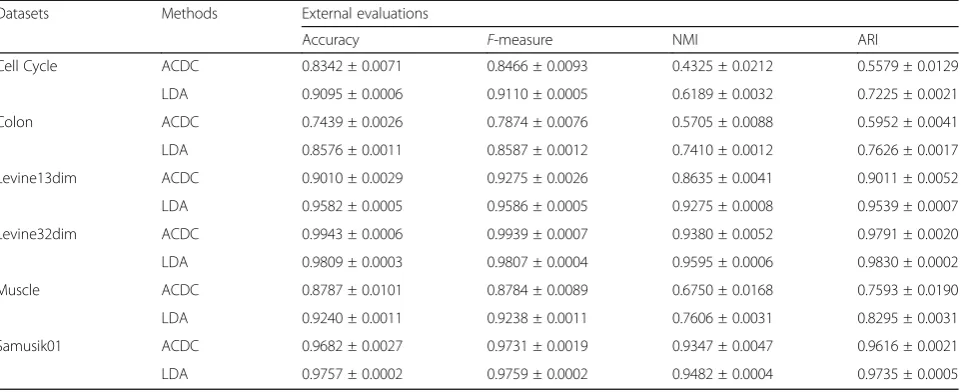
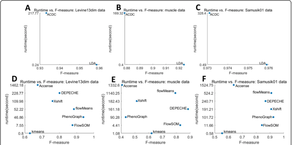
[image:3.595.55.537.99.304.2]Table 2 summarizes the comparison results of supervised methods. As expected, the two semi-supervised methods showed better performance than unsupervised methods (Table 3). In all datasets, both ACDC and LDA had greater accuracy,F-measure, NMI, and ARI than all unsupervised methods. This observa-tion is most noticeable in Cell Cycle data (F-measure > 0.82 vs.F-measure = 0.2–0.68), where the number of fea-tures [32] is significantly larger than the number of la-bels [4]. Next, we found that in all datasets except for Levine32dim, LDA had moderately better performance than ACDC. The significant lower runtime of LDA (Fig. 1 and Additional file 1: Figure S2) also indicates
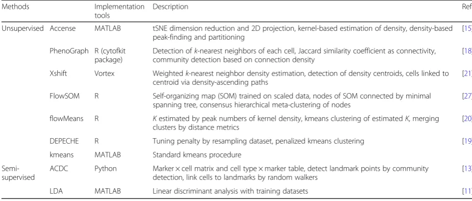
Table 1Methods compared in the study
Methods Implementation tools
Description Ref
Unsupervised Accense MATLAB tSNE dimension reduction and 2D projection, kernel-based estimation of density, density-based peak-finding and partitioning
[15]
PhenoGraph R (cytofkit package)
Detection ofk-nearest neighbors of each cell, Jaccard similarity coefficient as connectivity, community detection based on connection density
[18]
Xshift Vortex Weightedk-nearest neighbor density estimation, detection of density centroids, cells linked to centroid via density-ascending paths
[21]
FlowSOM R Self-organizing map (SOM) trained on scaled data, nodes of SOM connected by minimal spanning tree, consensus hierarchical meta-clustering of nodes
[27]
flowMeans R Kestimated by peak numbers of kernel density, kmeans clustering of estimatedK, merging clusters by distance metrics
[20]
DEPECHE R Tuning penalty by resampling dataset, penalized kmeans clustering [19]
kmeans MATLAB Standard kmeans procedure
Semi-supervised
ACDC Python Marker × cell matrix and cell type × marker table, detect landmark points by community detection, link cells to landmarks by random walkers
[13]
that LDA may be the top choice for the task of reprodu-cing manual labels.
Although LDA is superior to ACDC in terms of precision, we all know that the precision of semi-supervised tool relies more on the availability of prior information. Since a training set is only necessary for
LDA but not for ACDC, which requires a
“marker × cell type” table instead, it is questionable whether LDA can still outperform ACDC when the training set is less sufficient. To answer this question, we first trained LDA with only a limited proportion of samples (randomly choosing 20%, 40%, 60%, and 80% of all samples in colon dataset) as the training set. We observed that the performance of LDA stayed constant when the size of training set varied (Add-itional file 1: Figure S3). Then, we trained LDA with all the cells from healthy colon tissue in the colon dataset, and predicted the labels of all the remaining cells from polyps, early-stage cancer tissue, and late-stage cancer tissue. We then applied ACDC to the entire colon dataset as well as the subset excluding cells from healthy tissue (Additional file 1: Figure S3). The predicted result from LDA was then compared to that from ACDC. Under these conditions, the F -measure of LDA dropped from 0.85 to 0.73, which was not better than that of ACDC (0.80 for the entire dataset, 0.74 for the subset excluding cells from healthy tissue). Similar tests were repeated on the Cell Cycle dataset with consistent results (Additional file 1: Figure S3): when only one cell line (THP, HELA, or 293 T) was chosen as the training set, LDA could not precisely classify samples from other cell lines. Thus, we concluded that LDA can be regarded as the opti-mal semi-supervised tool as long as the training set and the test set are homogenous.
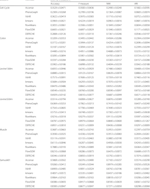
External evaluations of unsupervised tools highlight the precision of FlowSOM and flowMeans
Next, we performed external evaluation for seven un-supervised methods and observed that the precisions of different tools varied among different datasets. Com-pared to other methods, FlowSOM had relatively high precision values among all datasets (Table3). In the Cell Cycle dataset, FlowSOM was the only unsupervised tool that had an F-measure larger than 0.5. FlowSOM also had a relative short runtime (Fig.1and Additional file1: Figure S2), which is another advantage to be considered when choosing a suitable tool. In other datasets, such as the muscle and colon datasets (Table3), flowMeans had similar precision to FlowSOM. In fact, flowMeans out-performed FlowSOM in Samusik01 data (ARI 0.92 vs. 0.85). However, PhenoGraph had the best performance in the Levine13dim (ARI 0.927) and Samusik01 (ARI 0.925) datasets but performed poorly in the muscle, Cell Cycle, and colon datasets. On the contrary, DEPECHE exhibited excellent performance in datasets with rela-tively small numbers of cell types such as Levine32dim (F-measure = 0.92), muscle (F-measure = 0.89), and colon (F-measure = 0.68). In summary, FlowSOM and flow-Means had overall better precisions in our external evaluation, followed by PhenoGraph and DEPECHE.
Internal evaluations indicate that DEPECHE, FlowSOM, and PhenoGraph best captured the inner structure of CyTOF data
[image:4.595.59.543.99.295.2]We have exploited external evaluation metrics to analyze whether a clustering tool can accurately reproduce the manual-gated labels as the “ground truth.”However, re-searchers often wish to partition cells based on the nat-ural structure of biomarker expression profile without considering any assumptions about cell partitions. Here,
Table 2Summary of external evaluations for semi-supervised methods
Datasets Methods External evaluations
Accuracy F-measure NMI ARI
Cell Cycle ACDC 0.8342 ± 0.0071 0.8466 ± 0.0093 0.4325 ± 0.0212 0.5579 ± 0.0129
LDA 0.9095 ± 0.0006 0.9110 ± 0.0005 0.6189 ± 0.0032 0.7225 ± 0.0021
Colon ACDC 0.7439 ± 0.0026 0.7874 ± 0.0076 0.5705 ± 0.0088 0.5952 ± 0.0041
LDA 0.8576 ± 0.0011 0.8587 ± 0.0012 0.7410 ± 0.0012 0.7626 ± 0.0017
Levine13dim ACDC 0.9010 ± 0.0029 0.9275 ± 0.0026 0.8635 ± 0.0041 0.9011 ± 0.0052
LDA 0.9582 ± 0.0005 0.9586 ± 0.0005 0.9275 ± 0.0008 0.9539 ± 0.0007
Levine32dim ACDC 0.9943 ± 0.0006 0.9939 ± 0.0007 0.9380 ± 0.0052 0.9791 ± 0.0020
LDA 0.9809 ± 0.0003 0.9807 ± 0.0004 0.9595 ± 0.0006 0.9830 ± 0.0002
Muscle ACDC 0.8787 ± 0.0101 0.8784 ± 0.0089 0.6750 ± 0.0168 0.7593 ± 0.0190
LDA 0.9240 ± 0.0011 0.9238 ± 0.0011 0.7606 ± 0.0031 0.8295 ± 0.0031
Samusik01 ACDC 0.9682 ± 0.0027 0.9731 ± 0.0019 0.9347 ± 0.0047 0.9616 ± 0.0021
LDA 0.9757 ± 0.0002 0.9759 ± 0.0002 0.9482 ± 0.0004 0.9735 ± 0.0005
Table 3Summary of external evaluations for unsupervised methods
Datasets Methods External evaluations
Accuracy F-measure NMI ARI
Cell Cycle Accense 0.3529 ± 0.0471 0.3500 ± 0.0636 0.2490 ± 0.0240 0.1682 ± 0.0395
PhenoGraph 0.2309 ± 0.0268 0.2789 ± 0.0196 0.1364 ± 0.0087 0.0683 ± 0.0074
Xshift 0.3622 ± 0.0419 0.3970 ± 0.0383 0.1710 ± 0.0165 0.0752 ± 0.0353
kmeans 0.3969 ± 0.0021 0.4224 ± 0.0019 0.0963 ± 0.0016 0.0681 ± 0.0016
flowMeans 0.3055 ± 0.0061 0.3506 ± 0.0051 0.1849 ± 0.0047 0.0694 ± 0.0058
FlowSOM 0.6605 ± 0.0021 0.6897 ± 0.0029 0.1040 ± 0.0035 0.1171 ± 0.0025
DEPECHE 0.2808 ± 0.0126 0.3551 ± 0.0110 0.1361 ± 0.0246 0.0546 ± 0.0197
Colon Accense 0.3209 ± 0.0353 0.3495 ± 0.0442 0.4504 ± 0.0286 0.2304 ± 0.0304
PhenoGraph 0.3772 ± 0.0201 0.3994 ± 0.0137 0.4254 ± 0.0073 0.2696 ± 0.0094
Xshift 0.3187 ± 0.0167 0.3094 ± 0.0124 0.3763 ± 0.0076 0.2399 ± 0.0299
kmeans 0.4480 ± 0.0216 0.4951 ± 0.0086 0.4688 ± 0.0073 0.3235 ± 0.0132
flowMeans 0.5095 ± 0.0894 0.5901 ± 0.0582 0.4705 ± 0.0619 0.3724 ± 0.1125
FlowSOM 0.5597 ± 0.0284 0.5888 ± 0.0230 0.5303 ± 0.0157 0.4157 ± 0.0288
DEPECHE 0.5902 ± 0.0186 0.6898 ± 0.0132 0.4694 ± 0.0239 0.5042 ± 0.0188
Levine13dim Accense 0.6055 ± 0.0946 0.6745 ± 0.0929 0.7486 ± 0.0603 0.6408 ± 0.1034
PhenoGraph 0.8880 ± 0.0015 0.9123 ± 0.0167 0.8639 ± 0.0078 0.8884 ± 0.0159
Xshift 0.7573 ± 0.0091 0.7606 ± 0.0125 0.7359 ± 0.0118 0.7465 ± 0.0116
kmeans 0.5684 ± 0.0504 0.6293 ± 0.0325 0.7070 ± 0.0193 0.5721 ± 0.0465
flowMeans 0.8470 ± 0.0486 0.8842 ± 0.0343 0.8352 ± 0.0282 0.8349 ± 0.0459
FlowSOM 0.8540 ± 0.0235 0.8760 ± 0.0200 0.8590 ± 0.0097 0.8732 ± 0.0168
DEPECHE 0.6929 ± 0.0142 0.8010 ± 0.0077 0.6687 ± 0.0099 0.6571 ± 0.0118
Levine32dim Accense 0.5514 ± 0.0794 0.6008 ± 0.0627 0.6876 ± 0.0389 0.5289 ± 0.0740
PhenoGraph 0.6369 ± 0.0253 0.7062 ± 0.0213 0.7410 ± 0.0142 0.6437 ± 0.0240
Xshift 0.7543 ± 0.0605 0.7706 ± 0.0469 0.7690 ± 0.0323 0.7593 ± 0.0737
kmeans 0.5753 ± 0.0413 0.6748 ± 0.0231 0.7302 ± 0.0115 0.6405 ± 0.0638
flowMeans 0.9216 ± 0.0318 0.9279 ± 0.0337 0.9115 ± 0.0290 0.9397 ± 0.0342
FlowSOM 0.8787 ± 0.0975 0.8979 ± 0.0664 0.8840 ± 0.0600 0.8803 ± 0.1267
DEPECHE 0.8931 ± 0.0010 0.9231 ± 0.0009 0.8436 ± 0.0008 0.9297 ± 0.0009
Muscle Accense 0.3687 ± 0.0663 0.4072 ± 0.0743 0.3953 ± 0.0391 0.2397 ± 0.0759
PhenoGraph 0.3930 ± 0.0325 0.4336 ± 0.0249 0.3912 ± 0.0083 0.2694 ± 0.0261
Xshift 0.5119 ± 0.0591 0.5133 ± 0.0463 0.3882 ± 0.0190 0.3572 ± 0.0405
kmeans 0.6113 ± 0.0046 0.6207 ± 0.0045 0.4958 ± 0.0030 0.4243 ± 0.0055
flowMeans 0.7880 ± 0.0193 0.7928 ± 0.0089 0.5841 ± 0.0145 0.6364 ± 0.0347
FlowSOM 0.8210 ± 0.0068 0.8286 ± 0.0073 0.6470 ± 0.0072 0.6688 ± 0.0175
DEPECHE 0.8346 ± 0.0018 0.8850 ± 0.0019 0.5792 ± 0.0015 0.7074 ± 0.0035
Samusik01 Accense 0.5868 ± 0.0502 0.6376 ± 0.0400 0.7165 ± 0.0237 0.5574 ± 0.0290
PhenoGraph 0.9260 ± 0.0412 0.9249 ± 0.0344 0.8979 ± 0.0285 0.9250 ± 0.0526
Xshift 0.8909 ± 0.0485 0.9091 ± 0.0324 0.8742 ± 0.0196 0.8781 ± 0.0561
kmeans 0.4837 ± 0.0572 0.5535 ± 0.0401 0.6437 ± 0.0186 0.4655 ± 0.0482
flowMeans 0.9064 ± 0.0163 0.9099 ± 0.0163 0.8818 ± 0.0137 0.9206 ± 0.0045
FlowSOM 0.8386 ± 0.0693 0.8417 ± 0.0668 0.8185 ± 0.0639 0.8561 ± 0.0732
DEPECHE 0.8300 ± 0.0047 0.8677 ± 0.0047 0.7271 ± 0.0050 0.8298 ± 0.0068
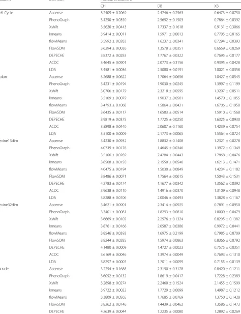
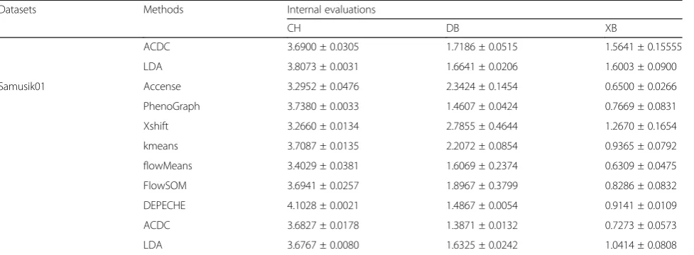
we analyzed the ability of a clustering tool to detect the inner structure of each dataset for the “coherence” as-sessment using three internal evaluations [33]—the Calinski-Harabasz index (CH, larger is better), Davies-Bouldin index (DB, smaller is better), and Xie-Beni index (XB, smaller is better)—in contrast to checking for re-producibility of sets of manual-gated labels by each tool. The detailed description of these indices is presented in the “Methods” section. These three internal evaluations have all been defined based on the assumption that an ideal cell partition should have both high within-group similarity and high between-group dissimilarity, which is exactly the characteristic that the natural clustering structure of CyTOF data should exhibit.
Table4shows that DEPECHE had noticeably high CH and low DB indices in all datasets and outperformed nearly all other tools. However, this observation should be interpreted with caution: CH and DB are indices that naturally favor kmeans-based algorithms [33], and the simple kmeans clustering also achieved high perform-ance based on CH and DB. Aside from DEPECHE and kmeans, PhenoGraph and FlowSOM also demonstrated good internal evaluation results over different datasets. PhenoGraph had the highest CH (larger is better), lowest DB (smaller is better), and third-lowest XB (smaller is better) in both the Levine13dim and Samusik01 datasets, whereas FlowSOM had the highest CH, lowest DB, and second-lowest XB in both the muscle and Cell Cycle datasets. In contrast to the above tools with consistent good results on all three indices, we observed inconsist-ency in the performance of Accense: it had the lowest
XB in the Levine13dim, muscle, Cell Cycle, and colon datasets but showed poor performance with respect to CH and DB. We reasoned that this inconsistency might be because XB naturally favors density-based algorithms [33]; hence, there is currently not enough evidence to state that Accense gives coherent clustering results.
A noteworthy fact is that unlike their strength in ex-ternal evaluation, semi-supervised tools no longer ranked top with respect to any of the internal evaluation indices. This result is consistent with the fact that even the manual labels themselves did not perform as well as top unsupervised tools in internal evaluation (Add-itional file 1: Table S3). Compared to LDA, ACDC showed better performance in internal evaluation. In some cases (DB and XB for Samusik01 and Levine32-dim, DB for Levine13Levine32-dim, etc.), the performance of ACDC was comparable with that of top-ranking un-supervised tools.
Given the above analysis, we recommended FlowSOM, PhenoGraph, and DEPECHE as preferred tools for the task of capturing inner structure of CyTOF data.
Stability evaluations suggest that PhenoGraph, DEPECHE, and LDA exhibited high robustness
[image:6.595.56.540.88.328.2]Table 4Summary of internal evaluations for each compared methods
Datasets Methods Internal evaluations
CH DB XB
Cell Cycle Accense 3.2409 ± 0.2069 2.4746 ± 0.2563 0.6473 ± 0.0750
PhenoGraph 3.4250 ± 0.0350 2.5692 ± 0.1503 0.7864 ± 0.0392
Xshift 3.5620 ± 0.0443 1.7337 ± 0.1618 0.9131 ± 0.3066
kmeans 3.9414 ± 0.0011 1.5971 ± 0.0013 0.7705 ± 0.0165
flowMeans 3.5992 ± 0.0283 1.6237 ± 0.0341 0.7294 ± 0.0393
FlowSOM 3.6294 ± 0.0036 1.3578 ± 0.0351 0.6669 ± 0.0269
DEPECHE 3.8372 ± 0.0283 1.7767 ± 0.0322 0.7695 ± 0.0177
ACDC 3.4645 ± 0.0901 2.0773 ± 0.3156 0.9395 ± 0.0428
LDA 3.4581 ± 0.0036 2.5080 ± 0.0191 1.0021 ± 0.0358
Colon Accense 3.2688 ± 0.0622 1.7064 ± 0.0656 1.0427 ± 0.0545
PhenoGraph 3.4231 ± 0.0194 1.9030 ± 0.0245 1.3997 ± 0.1199
Xshift 3.0706 ± 0.0179 2.3218 ± 0.0595 1.3207 ± 0.0511
kmeans 3.5109 ± 0.0079 1.9037 ± 0.0501 1.4570 ± 0.1055
flowMeans 3.4793 ± 0.1068 1.5864 ± 0.0421 1.6706 ± 0.1958
FlowSOM 3.6435 ± 0.0117 1.6583 ± 0.0514 1.5910 ± 0.1568
DEPECHE 3.9819 ± 0.0375 1.7725 ± 0.0250 1.6325 ± 0.0930
ACDC 3.5898 ± 0.0440 2.0607 ± 0.1160 1.4239 ± 0.0754
LDA 3.5100 ± 0.0009 2.1773 ± 0.0065 1.5564 ± 0.0724
Levine13dim Accense 3.4230 ± 0.0932 1.8832 ± 0.1408 1.2321 ± 0.0278
PhenoGraph 4.0739 ± 0.0176 1.4645 ± 0.0346 1.3972 ± 0.1349
Xshift 3.5106 ± 0.0289 2.4284 ± 0.0443 1.7868 ± 0.0476
kmeans 3.8508 ± 0.0150 2.1550 ± 0.0546 1.6213 ± 0.1471
flowMeans 4.0475 ± 0.0194 1.5030 ± 0.0849 1.4234 ± 0.1182
FlowSOM 3.8486 ± 0.0071 1.7564 ± 0.0615 1.5043 ± 0.1531
DEPECHE 4.2783 ± 0.0174 1.1677 ± 0.0342 1.3562 ± 0.0392
ACDC 3.9638 ± 0.0110 1.4916 ± 0.0370 1.3109 ± 0.0948
LDA 3.8288 ± 0.0106 2.0046 ± 0.0493 1.3828 ± 0.1167
Levine32dim Accense 3.4621 ± 0.0901 2.3414 ± 0.0925 0.7891 ± 0.0950
PhenoGraph 3.7401 ± 0.0081 1.8293 ± 0.0810 1.0009 ± 0.0479
Xshift 3.6669 ± 0.0102 2.2576 ± 0.1324 0.8295 ± 0.1382
kmeans 3.8761 ± 0.0166 2.0587 ± 0.0386 0.9972 ± 0.0441
flowMeans 3.8546 ± 0.0393 1.6975 ± 0.2199 0.7985 ± 0.0709
FlowSOM 3.8244 ± 0.0285 1.5974 ± 0.0863 0.8366 ± 0.0792
DEPECHE 4.1480 ± 0.0009 1.4727 ± 0.0023 0.7575 ± 0.0351
ACDC 3.6169 ± 0.0046 1.3974 ± 0.0049 0.7693 ± 0.1310
LDA 3.8297 ± 0.0007 1.7011 ± 0.0099 0.7155 ± 0.0139
Muscle Accense 3.2254 ± 0.1688 2.3190 ± 0.3178 0.8420 ± 0.1211
PhenoGraph 3.6052 ± 0.0132 1.8619 ± 0.0417 1.7228 ± 0.2389
Xshift 3.2898 ± 0.0274 2.2460 ± 0.1524 2.1455 ± 0.1599
kmeans 3.9722 ± 0.0022 1.7729 ± 0.0099 1.4987 ± 0.1212
flowMeans 3.3809 ± 0.0565 1.7685 ± 0.0769 1.3750 ± 0.1428
FlowSOM 3.8262 ± 0.0146 1.4439 ± 0.0462 1.3586 ± 0.1473
subsampling datasets, for testing; (2) directly given dif-ferent subsampling sizes, ranging from 5000 cells to 80, 000 cells, for testing. Then, we explored the robustness of each tool with respect to the number of identified clusters with varying sampling sizes.
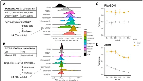
When considering the performance of a clustering tool, although its ability to cluster data into different meaningful populations is of great significance, its stabil-ity (or robustness) is also important. Therefore, we mea-sured the robustness against a fixed subsampling size by using the coefficient of variation (CV, smaller indicates better stability), and we measured the robustness against varying sample sizes by using the relative difference (RD, close to zero indicates better stability) between 20,000 cell tests (Additional file 2) and 40,000 cell tests (Ta-bles 2, 3, and 4, also see the “Methods” section). As shown in Fig.2a and Additional file1: Figure S4A, both semi-supervised tools and top-performing unsupervised tools had a high robustness against random subsamp-ling: median CVs for external evaluation in all datasets ranged from 0.001 (LDA) to 0.054 (Xshift), whereas those for internal evaluation ranged from 0.010 (LDA and DEPECHE) to 0.049 (flowMeans). A few extreme CV values for Xshift (ARI in CC data 0.46), DEPECHE (ARI in CC data 0.36), and flowMeans (ARI in colon data 0.31) indicate that performance of these tools might decline in specific cases. Thus, we observed that LDA had the best stability (largest CV for external evalu-ation < 0.006; largest CV for internal evaluevalu-ation = 0.08), followed by PhenoGraph (largest CV for external evalu-ation = 0.11; largest CV for internal evaluevalu-ation < 0.14).
By comparing the impact of varying sampling sizes on each tool (Fig.2b and Additional file1: Figure S4B), we observed that LDA, ACDC, DEPECHE, and PhenoGraph did not have large differences when the sample size ex-panded from 20,000 to 40,000. They all had a relative
difference (RD, see the “Methods” section) close to zero for all datasets. Xshift and FlowSOM exhibited some in-stability: the distribution of RD for Xshift was biased to-ward negative numbers, indicating that the precision of Xshift declined as sample size grew large. Although RD of FlowSOM was consistently around zero, there were some extreme values: RD for ARI in Samusik01 data was 0.38, whereas that in muscle data was 0.27. Similar re-sults were obtained from RD of internal evaluation met-rics (Additional file 1: Figure S4B). Since flowMeans frequently introduced singularity errors with a sample size of less than or equal to 20,000 (data not shown), we did not consider testing on flowMeans.
To further investigate the influence of sample size on Xshift and FlowSOM, we carried out additional sub-sampling tests (random sub-sampling of 5000, 10,000, 60, 000, and 80,000 cells). In both the Levine32dim and colon datasets,F-measure of Xshift dropped significantly as the sample size grew large. Although averageF -meas-ure of FlowSOM was relatively stable across different sample sizes, the standard deviation of F-measure reached a minimum when sample size reached a max-imum (80,000 cells in both datasets), indicating that FlowSOM was more robust at analyzing large datasets (Fig.2c, d).
PhenoGraph and Xshift detect more clusters, especially with a large sample size
[image:8.595.58.547.99.279.2]We believed that the robustness of a method should be evaluated by the stability of not only the performance of clustering but also the number of identified clusters. Therefore, we further explored the robustness of methods with respect to the number of identified clusters with varying sampling sizes. Since four of the tested tools (ACDC, LDA, kmeans, and FlowSOM) take the number of clusters as a required known Table 4Summary of internal evaluations for each compared methods(Continued)
Datasets Methods Internal evaluations
CH DB XB
ACDC 3.6900 ± 0.0305 1.7186 ± 0.0515 1.5641 ± 0.15555
LDA 3.8073 ± 0.0031 1.6641 ± 0.0206 1.6003 ± 0.0900
Samusik01 Accense 3.2952 ± 0.0476 2.3424 ± 0.1454 0.6500 ± 0.0266
PhenoGraph 3.7380 ± 0.0033 1.4607 ± 0.0424 0.7669 ± 0.0831
Xshift 3.2660 ± 0.0134 2.7855 ± 0.4644 1.2670 ± 0.1654
kmeans 3.7087 ± 0.0135 2.2072 ± 0.0854 0.9365 ± 0.0792
flowMeans 3.4029 ± 0.0381 1.6069 ± 0.2374 0.6309 ± 0.0475
FlowSOM 3.6941 ± 0.0257 1.8967 ± 0.3799 0.8286 ± 0.0832
DEPECHE 4.1028 ± 0.0021 1.4867 ± 0.0054 0.9141 ± 0.0109
ACDC 3.6827 ± 0.0178 1.3871 ± 0.0132 0.7273 ± 0.0573
LDA 3.6767 ± 0.0080 1.6325 ± 0.0242 1.0414 ± 0.0808
input, we only investigated the robustness of the other five tools (Accense, PhenoGraph, flowMeans, Xshift, and DEPECHE).
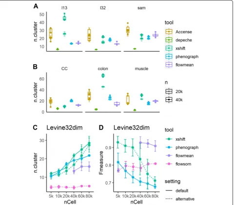
As shown in Fig. 3a, b, DEPECHE detected a small number of clusters in all datasets with little deviation. In all datasets and sample sizes, the number of clusters identified by DEPECHE ranged between 3 and 8. On the contrary, Xshift detected more clusters compared to all other tools. As the sample size grew from 20,000 to 40, 000, the number of clusters identified by Xshift also grew significantly. PhenoGraph also identified a rela-tively large number of clusters in the Levine32dim, Cell Cycle, and colon datasets and was moderately impacted by sample size in the Samusik01 and colon datasets. The number of clusters detected by flowMeans was not as extreme as DEPECHE or Xshift but was more inconsist-ent compared to DEPECHE, Xshift, and PhenoGraph in 40,000 cells subsampling tests.
Given that PhenoGraph and Xshift identified more clusters and that flowMeans was more inconsistent than the above two tools, we carried out further subsampling tests for PhenoGraph, Xshift, and flowMeans to evaluate the influence of sample size on robustness. Since Xshift provides an alternative way to determine the parameter K in KNN called Elbow Plot Determination, we carried
out further Xshift analysis using the Elbow Plot method to see whether it could give a stable result. Similarly, FlowSOM had an alternative option to estimate the number of clusters within a given range; hence, these two cases were also included in the comparison with vary-ing samplvary-ing sizes. As shown in Fig.3and Additional file1: Figure S5, the number of clusters detected by Xshift (de-fault fixed K) grew greatly as the sample size grew from 5000 to 80,000, and Xshift (with the alternative Elbow Plot setting) partly decreased this growth. However, the num-ber of clusters detected still grew faster when using Xshift with either setting than when using PhenoGraph. Further-more, for PhenoGraph and Xshift, the increase in the number of clusters accompanied a decline in precision (Fig. 3d). On the contrary, as the sample size grew, the precision for flowMeans declined without a significant change in the number of detected clusters. An interesting phenomenon is that when FlowSOM was forced to auto-matically determine the number of clusters, it stably iden-tified very few clusters just like DEPECHE did, but its precision was moderately lower than default setting (Fig.3d vs. Fig.2c). Comparing Fig.2c to Fig.3d, the pre-cision and the stability of FlowSOM consistently reached their peaks when the sampling size was at its maximum (80,000).
Fig. 2Stability of each tool.aLeft: schematic diagram showing how coefficients of variation (CVs) were calculated and integrated; right: distribution of CVs for external evaluations for each tool. The red solid line represents median CV for LDA, which is the smallest median CV.b
[image:9.595.55.538.87.361.2]Xshift and PhenoGraph identified refined sub-clusters of major cell types
Based on the above comparison analysis, we discovered several notable characteristics of Xshift and Pheno-Graph: (1) they had recognizable clustering structures (shown by better internal evaluation results), (2) they tended to overestimate the total number of clusters compared to the number defined by manual gating strat-egy, and (3) they exhibited reduced precision on datasets that had much smaller numbers of labels than numbers of features (muscle, Cell Cycle, colon). These character-istics suggested that Xshift and PhenoGraph tend to identify refined sub-clusters of major cell types. In other
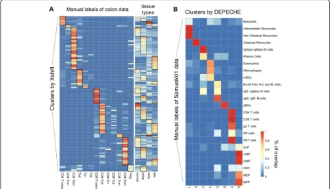
[image:10.595.60.541.88.509.2]alignment (Table 3). Since colon data involve samples originated from healthy tissue, polyps, early-stage cancer, and late-stage cancer, we tested whether Xshift discov-ered origin-specific patterns of cell clusters. We found that about three quarters (98 out of 132) of the clusters discovered by Xshift were origin-specific (more than 50% of cells come from the same sample origin) (Fig.4a). These results demonstrate that Xshift was able to classify specific subtypes of cells. Similar results were also found for PhenoGraph (Additional file 1: Figure S6A). How-ever, since PhenoGraph identified much smaller num-bers of clusters than Xshift (34 vs. 132, respectively), its capacity to recognize origin-specific clusters is relatively weaker than that of Xshift.
Next, DEPECHE also has an observable phenomenon that differentiates it from other tools. DEPECHE tended to underestimate the number of clusters and had better precision when the number of manual labels was small. We hypothesize that unlike Xshift and PhenoGraph, DEPECHE tends to group cells into major cell types. Carrying out the same analytical procedure as in Xshift but reversed, we obtained a one-to-many alignment be-tween DEPECHE clusters and the manual labels of the Samusik01 dataset (Fig. 4b). DEPECHE grouped differ-ent T cells into one cluster and six types of progenitor
cells into another. The difference among subtypes of B cells was also neglected by DEPECHE. We further found that in both the Samusik01 and Levine13dim (Add-itional file 1: Figure S6B) datasets, DEPECHE failed to recognize the characteristics of some small cell types such as basophil cells, eosinophil cells, nature killer cells, and subtypes of dendritic cells (Additional file 1: Figure S6B). All the above results demonstrate that DEPECHE is not suitable for analyzing refined subtypes.
Discussion
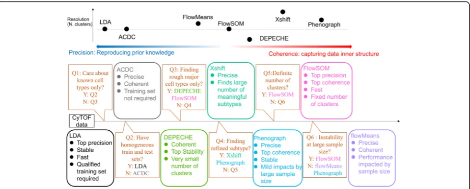
The aim of this study is to present a benchmark com-parison for current clustering methods for mass cytome-try data and to help researchers select the suitable tool based on the features of their specific data. To this end, we considered the precision (external comparison), co-herence (internal comparison), and stability of different clustering methods. As shown by our results, this com-parison procedure comprehensively depicts the charac-teristics of each tool, providing clear guidance for tool selection (Fig. 5). If researchers wish to determine the pros and cons of other existing or novel tools in the fu-ture, this benchmarking framework can be applied to make a thorough comparison.
[image:11.595.56.539.89.365.2]Semi-supervised tools fit the task of finding known clusters
As expected, both semi-supervised tools resulted in bet-ter performance in bet-terms of precision and stability than unsupervised approaches. This strength was observed in experiments with varying sample sizes, numbers of fea-tures, and different indicators (accuracy, F-measure, NMI, ARI), suggesting that the advantage of semi-supervised approaches in precision is dominant and ex-haustive. Thus, the ability to precisely and robustly re-produce manual labels makes semi-supervised tools suitable for situations where researchers focus on the known cell types with reliable prior knowledge.
The two semi-supervised tools compared in our study, LDA and ACDC, have a fundamental difference in terms of prior input knowledge: LDA requires a training set with manual labels as the input, whereas ACDC requires a“marker × cell type” table that defines the relationship between features and labels. This difference is vital for the choice of semi-supervised tools. In our study, LDA outperformed ACDC in most of the indicators, including precision, stability, and runtime, which made LDA the preferred tool in most conditions. However, LDA de-pends on a reliable, homogenous training set. When there is no available training set with manual labels, or the training set and test set are heterogeneous (i.e., sam-ples come from different tissues or cell lines, but train-ing set contains only one tissue/cell line), ACDC would be the better choice (Fig.5Q2).
Another interesting result is that the performance of semi-supervised tools was beaten by unsupervised tools with respect to coherence (internal evaluation), suggest-ing that definsuggest-ing cell types based on isolated markers might not precisely capture the inner structure of the
data. This observation is not surprising, considering that the number of bi-axal plots required to depict the rela-tionship among features increases exponentially as the number of features increases [12]. Using only dozens of bi-axal plots is thus unlikely to capture the whole pic-ture. The human-subjective judgment of manual gating [34] is another factor that hinders semi-supervised tools from characterizing the objective features of CyTOF data.
PhenoGraph and FlowSOM are the top-performing unsupervised tools
The manual gating of mass cytometry data requires heavy labor and results in issues regarding reproducibility and sub-jectivity. Efforts to reduce such burdens have given rise to a wide variety of unsupervised approaches that partition cell populations according to the natural structure of cell data [12]. Our results showed that two outstanding approaches, PhenoGraph and FlowSOM, gave more precise and coherent clustering results than other approaches. Each of these two approaches had an impressive ability to produce coherent clustering results; PhenoGraph showed higher stability, and FlowSOM had the highest precision. We suggest Pheno-Graph and FlowSOM as the two top-tier choices when re-searchers are looking to focus more on the inner structure of the data instead of relying on external prior knowledge.
[image:12.595.60.539.87.280.2]worsens the performance of FlowSOM. Furthermore, even if a large estimate range (up to twice the number manual labels) was provided, FlowSOM consistently selected a small number of clusters. We believe that the default set-ting (inputset-ting a predetermined number of clusters) is the optimal setting for FlowSOM, which partially limits the application of this promising tool.
Sample size has a vital impact
An essential challenge for CyTOF technology is that sample size can vary significantly among different CyTOF experiments [2]. Our results demonstrated that various tools exhibited different performance results when dealing with varying sample sizes; thus, sample size must be taken into consideration when choosing the appropriate tools.
As shown in Fig. 3, the number of clusters found by PhenoGraph and Xshift positively correlated to sample size. This trend could be alleviated, but not eliminated, by the usage of Elbow Plot Determination in Xshift. We reasoned that the impact of large sample size on the number of clusters might have arisen from the inner characteristics of density-based partitioning methods. Generally speaking, both the Louvain method and other modularity maximization algorithms aim to find the op-timal partition of a network that reaches a maximum “Newman-Girvan modularity,” or Qmax. However, the
maximization ofQsuffers from the problem of extreme degeneracy: there is typically an exponential number of distinct partitions that are close to the optimum [35]. As the size of the network grows, the number of local opti-mal solutions grows geometrically, veiling the desired optimal partition. Furthermore, the many locally optimal solutions are often topologically dissimilar [35], which gives rise to inconsistent outputs. This characteristic in-troduces the potential risk that PhenoGraph and Xshift may be overwhelmed by extremely large sample sizes.
The impact of sample size on flowMeans was inconsistent. In one case, the performance of flowMeans declined when sample size grew large (Fig.3); in another case, flowMeans frequently introduced the error of singularity and array di-mensions in R when the sample size was smaller than 40, 000. Although experienced users may modify the source R code to avoid these errors, we believe that this practice is not advisable for common researchers without extensive pro-gramming experience in R. Comparatively speaking, Flow-SOM had better precision and stability with large sample sizes and is the best alternative choice when dealing with large amounts of cells.
Clustering resolution varies among different tools
Clustering resolution, the ability to detect small and re-fined clusters, has seldom been evaluated by previous publications, partly because many parameter settings can
impact the number of clusters identified by each tool. By using the default settings for each tool, we found that each tool, as well as their different settings, had a dis-tinct tendency to over- or underestimate the number of clusters. This tendency should not be neglected, given the fact that an over- or underestimation is biologically significant (Fig. 4). Furthermore, the resolution of the manual label is more or less arbitrary and should not be regarded as“golden standard.” Thus, in most cases, the cell type resolution of CyTOF research is determined by the results of the chosen clustering tool.
In the current study, we found that PhenoGraph and Xshift output relatively larger numbers of clusters and split the manual clusters into smaller sub-clusters. On the contrary, DEPECHE grouped similar manual clusters into larger meta-clusters and ignored the subtle differ-ences among them. If researchers wish to focus on the refined subtypes of cells, the appropriate choice would be PhenoGraph or Xshift. If researchers cannot correctly estimate the number of refined clusters they are looking for, even FlowSOM would not be a good choice as Phe-noGraph or Xshift, as the small number of clusters found by automatic estimation of FlowSOM is not likely to be “refined”(Fig. 3). If Xshift and PhenoGraph suffer from instability with large sample sizes, an alternative strategy could be a primary application of FlowSOM or DEPECHE to obtain major cell types, followed by de-tailed sub-clustering on each major type.
Conclusions
Our study demonstrates that in the field of mass cytom-etry analysis, LDA best fits the task of precisely reprodu-cing manual clustering labels. PhenoGraph and FlowSOM are the top unsupervised tools because of their high precision, coherence, and stability. Pheno-Graph and Xshift can detect a refined subset of major cell types, whereas DEPECHE and FlowSOM tend to group similar cell types into large meta-clusters. Deci-sion guidance has been provided (Fig.5) as a concluding summary to facilitate the choice of suitable clustering tools based on users’specific situations.
Methods Clustering tools
ACDC are top-performance tools in a previous compari-son of semi-supervised tools by Abdelaal et al. [11]. kmeans clustering was implemented using a built-in MATLAB kmeans function. The remaining approaches were implemented using the original articles’ sugges-tions. All tools were freely available for use from the ori-ginal articles.
In general, we performed each algorithm on arcsinh-transformed data and with default settings. To minimize the influence of inconsistent transformation and scaling methods, we invalidated all transformation and scaling functions for all software (i.e., standardize = FALSE for flowMeans, transformation = NONE and rescale = NONE for Xshift). All the compared tools were per-formed on a single PC (Intel® Core™ i5-8400 CPU @ 2.80 GHz, a processor with 8.00 GB memory). By default, Xshift was run using standalone.bat with a minimum memory of 1 GB.
Datasets
We tested the performance of these nine tools on six mass cytometry datasets that served as “benchmarking datasets”(Additional file 1: Table S1). All of these data-sets were biologically well characterized with known cell-type annotations. Among them, Levine13dim, Levi-ne32dim, and Samusik01 are well-known benchmarking CyTOF datasets and have already been summarized by Weber and Robinson in their previous comparison [25]. The other three new datasets were summarized as follows:
1) Muscle-resident cells from healthy adult mice [28]. Twenty-five proteins were used for clustering. Eight major cell populations were identified according to provided gating strategies, including Neg/Neg cells that lacked any known cell markers.
2) In vitro cells from three cell lines—HEK293T, MDA-MB-231, and THP-1 [29]. These cell lines were treated by TNFαto induce a cell cycle trans-formation. Cells at different time points were col-lected after treatment. Cells were labeled by four phases: G0/G1, G2, S, and M. A total of 35 markers were measured.
3) Our laboratory’s private human colon data [36]. Cells were collected from healthy colon tissue, polyps of a healthy adult, early-stage colon cancer, and late-stage colon cancer. Nineteen protein markers were used for clustering, and 13 manual la-bels were generated using gating strategies.
Pre-processing of datasets
First of all, each dataset was filtered to remove annota-tion incompleteness, doublets, debris, and dead cells. Then, expression levels of all proteins were normalized
by the inverse hyperbolic sine function (denoted by arc-sinh) with a scale factor of 5:
expnormalized¼ arcsinh exp 5
All nine tools were applied on the filtered and normal-ized datasets.
Then, we realized that Levine13dim, Levine32dim, and Samusik01 datasets contained unassigned cells or cells with ambiguous annotations (denoted as “NaN” in each .fcs file), which did not belong to any manually gated populations. For this matter, some researchers would like to discard these unassigned cells since these cells were usually low quality cells, intermediate cells, or cells that did not express on some known markers [11, 23]. There were also some researchers who preferred to in-clude these unassigned cells into the clustering [18, 21]. As the existing researches have done, we did the further pre-processing for these three datasets in the following two ways:
1) We discarded unassigned cells or cells with ambiguous annotations and only clustered cells with manually gated annotations into different populations by the compared tools.
2) We executed each compared tools on all cells including unassigned cells or cells with ambiguous annotations, but calculated the evaluation measures using the subset of annotated cells.
By observing the results of both cases (discarding unassigned cells see Tables 2, 3, and 4, including un-assigned cells see Additional file 1: Table S4 and S5) separately, it was not difficult to find that the overall ranking order of compared methods was almost the same. However, comparing the results of each method between these two cases, we found that only unstable methods (such as Accense and Xshift) presented obvious changes, and the relatively stable methods ba-sically remained unchanged under our comparison framework (such as DEPECHE and ACDC). There-fore, we mainly discuss the result analysis for datasets excluding unassigned cells, and the results of includ-ing unassigned cells are presented in Additional file 1: Table S4 and S5.
Subsampling tests
Since different datasets contain different numbers of cells and analysis on large datasets is very time consum-ing, we randomly subsampled 20,000 and 40,000 cells (5 times each) from each dataset and applied all tools on them. The largest number of subsampling was set at 40, 000 because the Samusik01 dataset contains only 53,173 cells with manual annotations. Internal evaluations, ex-ternal evaluations, stability tests, and further down-stream analysis were conducted on these subsampled cells. To further analyze the impact of sample size on the performance of PhenoGraph, Xshift, FlowSOM, and flowMeans, we carried out additional subsampling tests with sample sizes of 5000, 10,000, 60,000, and 80,000 on 2 datasets: Levine32dim and colon. This was because these two datasets have over 100,000 cells and have moderate numbers of manual labels (14 for Levine32dim and 13 for colon).
An exception to this analysis was when the sample size was less than or equal to 20,000, where flowMeans in-troduced errors of singularity and array dimensions in more than half of the random sampling tests. We in-ferred that subsampling data without singularity errors might result in bias, so we did not carry out any tests on flowMeans with sample size of less than or equal to 20, 000.
Internal evaluations measure the homogeneity of clustering results
In the current study, we utilized both internal and exter-nal evaluations to measure the clustering performance of different approaches. Internal evaluations are based on the hypothesis that an ideal clustering result should have high similarity within each cluster and high heterogen-eity between clusters. These evaluations do not require additional “true labels” and analyze the internal charac-teristics of a clustering result. Such characcharac-teristics make them compatible to give a fair comparison between semi-supervised and unsupervised methods. Three in-ternal evaluation methods were adopted in our study:
1. The Xie-Beni index (XB) [32]. We first calculate the pooled within-group sum of squares (WGSS) which measure the dispersion within each cluster as:
WGSS¼X k
1
nk
X
i<j∈Ik
Mf gik −M k
f g j
2
Where Ik denotes all the samples in cluster k, nk=∣ Ik∣, and M
fkg
i represents the observation of samplei(for i∈Ik). We then calculate the between-cluster distance as:
δ1 k;k 0
¼ min
i∈Ik j∈Ik0
d Mi;Mj
whered(a,b) is the Euclidean distance betweenaandb. Based on the above two measurements, XB is defined as:
XB¼1
n
WGSS
min k<k0
δ1 k;k 0
2
2. The Calinski-Harabasz index (CH) [32]. CH also utilizes WGSS to measure the dispersion within each cluster. But unlike XB, CH uses another meas-urement, between-group sum of squares (BGSS), to measure dispersion between clusters:
BGSS¼X K
i¼1
nkGf gk −G
2
whereG{k}denotes the barycenter for clusterk, andGis the barycenter of all samples. Then, CH is defined as follows:
CH¼N−K
K−1
BGSS WGSS
3. The Davies-Bouldin index (DB) [32]. DB measures the dispersion within each cluster by average dis-tance to barycenter:
δk ¼
1
nk
X
i∈Ik
Mf gik −Gk
f g
whereas the dispersion between clusters is measured by:
Δkk0 ¼ Gf gk −G k 0
Integrating these measures, DB can be written as:
DB¼ 1
K
XK
k¼1
max k0≠k
δkþδk0
Δkk0 !
External evaluations measure the precision of clustering results
methods over unsupervised methods since they make use of the same true labels.
To measure the precision of predicted clustering, the first step is to obtain a one-to-one mapping between predicted clusters and true cell population. This was achieved by the Hungarian assignment algorithm, a combinatorial optimization algorithm that finds the as-signment with the lowest F-measure in true cell popula-tions [21]. Then, four different external evaluapopula-tions were adopted:
1. Single cell-level accuracy (AC) [31], which is de-fined as the ratio of correctly clustered cells in total cells. Supposenis the total number of cells,Mis the vector of cluster labels annotated by manual gating, andTis the vector of cluster labels pre-dicted by tested approaches. map(Ti) is the one-to-one mapping between predicted clusters and actual cell cluster achieved by the Hungarian assignment algorithm. AC is calculated by:
AC¼1
n
Xn
i¼1
δðMi;mapð ÞTi Þ
where
δðx;yÞ ¼ 1;0;if x¼y;
if x≠y
2. WeightedF-measure (harmonic mean of precision and recall) [37]. For each clusteri, we use
Fi¼
2PiRi
PiþRi
to calculate its F-measure, where Pi¼ true positive
true positiveþfalse positive and Ri¼true positiveþfalse negativetrue positive
repre-sent precision and recall of clusteri. We summed up the
F-measure of each cluster over all clusters to obtain the weightedF-measure:
F¼Xni
NFi
wherenirepresent the number of cells in clusteriandN
represents the total number of cells.
3. Normalized Mutual Information (NMI) [30]. Supposem∈Mis the clustering assignment from manual gating,t∈Tis the clustering assignment from the tested approach,PM(m) andPT(t) are their probability distributions, andPMT(m,t) is their joint
distribution. Their information entropies are calculated by:
H Mð Þ ¼−X
m
pMð Þm logPMð Þm
H Tð Þ ¼−X
t
pTð Þt logPTð Þt
We defined mutual information (MI) ofMandTas:
I Mð ;TÞ ¼X
m;t
PMTðm;tÞlog PMT m;t
ð Þ
pMð Þm pTð Þt
If we treat bothMand Tas discrete random variables, their statistical redundancy reflects the clustering accur-acy (note that a perfect clustering result T and the true labelsM are completely redundant because they contain the same information).I(M,T) captures this redundancy, but its normalized form:
NMI¼ 2I Mð ;TÞ
H Mð Þ þH Tð Þ
is a more commonly used evaluation. The value of NMI would be large ifTis an optimal clustering result. In an ideal situation,T=Mcorresponds to NMI = 1.
4. Adjusted Rand Index (ARI) [38]. Given two different partitions of a same set of samples,Xi(1≤
i≤r) andYj(1≤j≤s), we denotenijas the number of samples that are in bothXiandYj,nij= |Xi∩Yj|. Letai¼
Ps
j¼1nijandbj¼ Pr
i¼1nij, we have ∑ai= ∑bj=∑nij=n. We can define ARI as:
ARI¼ P ij nij 2 − P i ai 2 P j bj 2 = n 2 1 2 X i ai 2 þ X j bj 2
− Xi ai
2 X j bj 2 = n 2
which measures the similarity between partition X and
Y.
Evaluation of stability
CV¼Standard Deviation Mean
For each tool, there were 24 CVs for external evalu-ation (6 datasets and 4 indices). Their distribution was calculated as a ridge plot (Fig.2), and we compared the robustness among tools by comparing the median and extreme values of the distribution of CVs.
The evaluation of robustness against varying sample size was conducted similarly, except that CV was re-placed by relative difference (RD) between 20,000 and 40,000 cell subsampling tests. For any given tool, dataset, and index, RD was defined as:
RD¼ðmean40k−mean20kÞ mean20k
Evaluation of the number of clusters
Among the nine tools we compared, kmeans, FlowSOM, LDA, and ACDC required the number of clusters as an input, flowMeans by default did not require this input, and the remaining tools automatically estimated the number of clusters. To test the stability of each tool, we recorded the number of clusters obtained by flowMeans, PhenoGraph, Accense, Xshift, and DEPECHE in each subsampling test. The standard deviation for each tool was calculated to represent the stability of the tool.
For FlowSOM and Xshift, there are widely applied al-ternative settings that impacted the number of detected clusters: Elbow Plot Determination to estimate K for KNN (Xshift) and automatic estimation of the number of clusters (FlowSOM). We evaluated the perfor-mances using these settings, together with Pheno-Graph and flowMeans, on the Levine32dim and colon datasets. For FlowSOM, the cluster number estima-tion range was set at 1 to 2 times the number of manual labels. This range proved to be wide enough given the fact that FlowSOM consistently estimated a relatively low number of clusters.
Evaluation of clustering resolution
To evaluate the ability of Xshift and PhenoGraph to find refined sub-clusters of manual labels, we defined a many-to-one alignment between predicted clusters and manual labels: if more than half of cells from a predicted cluster belonged to one manual label, we considered this predicted cluster to be a sub-cluster of the correspond-ing manual label. Under this alignment, we recalculated the F-measure, NMI, and ARI. To verify whether Xshift and PhenoGraph can resolve heterogeneity in sample origin in colon data, we defined that one predicted clus-ter is origin-specific if more than half of its cells come from one sample origin (normal tissue, polyps, early-stage cancer, or late-early-stage cancer). The fact that most of
the predicted clusters can be aligned to one manual label and that this alignment significantly improved precision demonstrates that Xshift and PhenoGraph indeed found the sub-clusters of manual labels. The fact that the majority of Xshift clusters were origin-specific demon-strates that Xshift is capable of resolving heterogeneity of sample origin.
Supplementary information
Supplementary informationaccompanies this paper athttps://doi.org/10. 1186/s13059-019-1917-7.
Additional file 1:Supplementary Method.Table S1.Data sets tested in the study.Table S2.Impacts of different transformation methods.Table S3.Internal evaluation for manual labels.Table S4.Summary of external evaluations including unassigned cells.Table S5. Summary of internal evaluations including unassigned cells.Figure S1.Flowchart of the study.
Figure S2.Runtime and F-measure of semi-supervised tools (A-C) and unsupervised tools (D-F) on Levine32dim, Cell Cycle and colon data sets.
Figure S3.Impact of limited training sets on the performance of LDA.
Figure S4.Stability of each tool evaluated by internal evaluations.Figure S5.Evaluation of impacts of sample size on colon data.Figure S6. Clus-tering resolution for PhenoGraph (colon data) and DEPECHE (Levine13-dim data).Figure S7.Gating strategy for colon data.
Additional file 2.Supplementary data.
Additional file 3.Review history.
Acknowledgements
Not applicable.
Peer review information
Yixin Yao was the primary editor on this article and managed its editorial process and peer review in collaboration with the rest of the editorial team.
Review history
The review history is available as Additional file3.
Authors’contributions
XD designed the study. XD and GNL supervised the study. XL and SY collected the data and tested methods. TZ generated and processed the private data. BW, XL, and WS conducted the study. XL and WS analyzed the data and wrote the manuscript. XD and GNL revised the manuscript. All authors read and approved the manuscript.
Funding
This work is supported by the Shanghai Municipal Science and Technology (2017SHZDZX01), National Natural Science Foundation of China (81871448, 81671328), National Key Research and Development Program of China (2017ZX10203205-006-002), Innovation Research Plan supported by Shanghai Municipal Education Commission (ZXWF082101), National Key R&D Program of China (2017YFC0909200), and Program for Professor of Special
Appointment (Eastern Scholar) at Shanghai Institutions of Higher Learning (1610000043).
Availability of data and materials
The Levine13dim, Levine32dim, and Samusik01 datasets are available in the “flowrepository”repository,http://flowrepository.org/id/FR-FCM-ZZPH. The muscle dataset is available athttps://community.cytobank.org/cytobank/ experiments/81774. The Cell Cycle dataset is available athttps://community. cytobank.org/cytobank/experiments/68981. The private colon cancer dataset is available athttp://flowrepository.org/id/FR-FCM-Z27K. All codes necessary for the current study are available athttps://github.com/WeiCSong/ cytofBench[39].
Ethics approval and consent to participate
Consent for publication
Not applicable.
Competing interests
The authors declare that they have no competing interests.
Author details
1State Key Laboratory of Oncogenes and Related Genes, Institute for
Personalized Medicine, School of Biomedical Engineering, Shanghai Jiao Tong University, 1954 Huashan Road, Shanghai 200030, China.2Shanghai Key
Laboratory of Psychotic Disorders, Shanghai Mental Health Center, Shanghai Jiao Tong University School of Medicine, 600 South Wanping Road, Shanghai 200030, China.3Department of Biomedical Engineering, Johns Hopkins University, Baltimore, MD 21218, USA.
Received: 15 August 2019 Accepted: 9 December 2019
References
1. Stuart T, Satija R. Integrative single-cell analysis. Nat Rev Genet. 2019;20:257– 72.
2. Spitzer MH, Nolan GP. Mass cytometry: single cells, many features. Cell. 2016;165:780–91.
3. Anchang B, Davis KL, Fienberg HG, Williamson BD, Bendall SC, Karacosta LG, et al. DRUG-NEM: optimizing drug combinations using single-cell perturbation response to account for intratumoral heterogeneity. Proc Natl Acad Sci. 2018;115:E4294–303.
4. Reeves PM, Sluder AE, Paul SR, Scholzen A, Kashiwagi S, Poznansky MC. Application and utility of mass cytometry in vaccine development. FASEB J. 2018;32:5–15.
5. Bader L, Gullaksen S-E, Blaser N, Brun M, Bringeland GH, Sulen A, et al. Candidate markers for stratification and classification in rheumatoid arthritis. Front Immunol. 2019;10:1488.
6. Saadatpour A, Guo G, Orkin SH, Yuan G-C. Characterizing heterogeneity in leukemic cells using single-cell gene expression analysis. Genome Biol. 2014; 15:525.
7. Bacher R, Kendziorski C. Design and computational analysis of single-cell RNA-sequencing experiments. Genome Biol. 2016;17:63.
8. Stoeckius M, Zheng S, Houck-Loomis B, Hao S, Yeung BZ, Mauck WM, et al. Cell hashing with barcoded antibodies enables multiplexing and doublet detection for single cell genomics. Genome Biol. 2018;19:224.
9. Bandura DR, Baranov VI, Ornatsky OI, Antonov A, Kinach R, Lou X, et al. Mass cytometry: technique for real time single cell multitarget immunoassay based on inductively coupled plasma time-of-flight mass spectrometry. Anal Chem American Chemical Society. 2009;81:6813–22.
10. Diggins KE, Ferrell PB, Irish JM. Methods for discovery and characterization of cell subsets in high dimensional mass cytometry data. Methods. 2015;82: 55–63.
11. Abdelaal T, van Unen V, Höllt T, Koning F, Reinders MJT, Mahfouz A. Predicting cell populations in single cell mass cytometry data. Cytom Part A; 2019;95:769–81.
12. Mair F, Hartmann FJ, Mrdjen D, Tosevski V, Krieg C, Becher B. The end of gating? An introduction to automated analysis of high dimensional cytometry data. Eur J Immunol. 2016;46:34–43.
13. Lee H-C, Kosoy R, Becker CE, Dudley JT, Kidd BA. Automated cell type discovery and classification through knowledge transfer. Bioinformatics. 2017;33:1689–95.
14. Pezzotti N, Lelieveldt BPF, van der Maaten L, Hollt T, Eisemann E, Vilanova A. Approximated and user steerable tSNE for progressive visual analytics. IEEE Trans Vis Comput Graph. 2017;23:1739–52.
15. Shekhar K, Brodin P, Davis MM, Chakraborty AK. Automatic classification of cellular expression by nonlinear stochastic embedding (ACCENSE). Proc Natl Acad Sci U S A Natl Acad Sci. 2014;111:202–7.
16. Chen H, Lau MC, Wong MT, Newell EW, Poidinger M, Chen J. Cytofkit: a bioconductor package for an integrated mass cytometry data analysis pipeline. PLOS Comput Biol. 2016;12:e1005112.
17. Amir ED, Davis KL, Tadmor MD, Simonds EF, Levine JH, Bendall SC, et al. viSNE enables visualization of high dimensional single-cell data and reveals phenotypic heterogeneity of leukemia. Nat Biotechnol. 2013;31:545–52.
18. Levine JH, Simonds EF, Bendall SC, Davis KL, Amir ED, Tadmor MD, et al. Data-driven phenotypic dissection of AML reveals progenitor-like cells that correlate with prognosis. Cell. 2015;162:184–97.
19. Theorell A, Bryceson YT, Theorell J. Determination of essential phenotypic elements of clusters in high-dimensional entities-DEPECHE. PLoS One. 2019; 14:e0203247.
20. Aghaeepour N, Nikolic R, Hoos HH, Brinkman RR. Rapid cell population identification in flow cytometry data. Cytom Part A. 2011;79A:6–13. 21. Samusik N, Good Z, Spitzer MH, Davis KL, Nolan GP. Automated mapping of
phenotype space with single-cell data. Nat Methods. 2016;13:493–6. 22. Biau G, Chazal F, Cohen-Steiner D, Devroye L, Rodríguez C. A weighted
k-nearest neighbor density estimate for geometric inference. Electron J Stat. 2011;5:204–37.
23. Wagner J, Rapsomaniki MA, Chevrier S, Anzeneder T, Langwieder C, Dykgers A, et al. A single-cell atlas of the tumor and immune ecosystem of human breast cancer. Cell Elsevier; 2019;0.
24. Porpiglia E, Samusik N, Van Ho AT, Cosgrove BD, Mai T, Davis KL, et al. High-resolution myogenic lineage mapping by single-cell mass cytometry. Nat Cell Biol. 2017;19:558–67.
25. Weber LM, Robinson MD. Comparison of clustering methods for high-dimensional single-cell flow and mass cytometry data. Cytom Part A. 2016; 89:1084–96.
26. Melchiotti R, Gracio F, Kordasti S, Todd AK, de Rinaldis E. Cluster stability in the analysis of mass cytometry data. Cytom Part A. 2017;91:73–84. 27. Van Gassen S, Callebaut B, Van Helden MJ, Lambrecht BN, Demeester P,
Dhaene T, et al. FlowSOM: using self-organizing maps for visualization and interpretation of cytometry data. Cytom Part A. 2015;87:636–45. 28. Giordani L, He GJ, Negroni E, Sakai H, Law JYC, Siu MM, et al.
High-dimensional single-cell cartography reveals novel skeletal muscle-resident cell populations. Mol Cell. 2019;74:609–21 e6.
29. Rapsomaniki MA, Lun X-K, Woerner S, Laumanns M, Bodenmiller B, Martínez MR. CellCycleTRACER accounts for cell cycle and volume in mass cytometry data. Nat Commun. Nat Publ Group; 2018;9:632.
30. Danon L, Díaz-Guilera A, Duch J, Arenas A. Comparing community structure identification. J Stat Mech Theory Exp. 2005;2005:P09008.
31. Liu H, Wu Z, Cai D, Huang TS. Constrained nonnegative matrix factorization for image representation. IEEE Trans Pattern Anal Mach Intell. 2012;34:1299–311. 32. Maulik U, Bandyopadhyay S. Performance evaluation of some clustering
algorithms and validity indices. IEEE Trans Pattern Anal Mach Intell. 2002;24: 1650–4.
33. Hassani M, Seidl T. Using internal evaluation measures to validate the quality of diverse stream clustering algorithms. Vietnam J Comput Sci. 2017; 4:171–83.
34. Maecker HT, McCoy JP, Nussenblatt R. Standardizing immunophenotyping for the Human Immunology Project. Nat Rev Immunol. 2012;12:191–200. 35. Good BH, de Montjoye Y-A, Clauset A. Performance of modularity
maximization in practical contexts. Phys Rev E. 2010;81:46106.
36. Zhang T, Lv J, Tan Z, Wang B, Warden AR, Li Y, et al. Immunocyte profiling using single-cell mass cytometry reveals EpCAM+ CD4+ T cells abnormal in colon cancer. Front Immunol. 2019;10:1571.
37. Hripcsak G, Rothschild AS. Agreement, the F-measure, and reliability in information retrieval. J Am Med Informatics Assoc Narnia. 2005;12:296–8. 38. Santos JM, Embrechts M. On the use of the adjusted Rand index as a metric
for evaluating supervised classification. Berlin: Springer; 2009. p. 175–84 39. Liu, Xiao. Song, Weichen. Wong, Brandon. Zhang, Ting. Yu, Shunying. Lin,
Guan Ning. Ding, Xianting. WeiCSong/cytofBench: a comparison framework and guideline of clustering methods for mass cytometry data (version v1.0). GitHub.https://github.com/WeiCSong/cytofBench(2019)).
Publisher’s Note