Obtaining an Accurate and Comprehensive
Data Mining Model
Anupa Sinha1, Dr.S.K.Shrivastava2
1
MPHIL Scholar, 2Professor
1
Dr.C.V.Raman University, Bilaspur, India,
2
Rajeev Gandhi Govt.P.G.College, Ambikapur (Surguja)
Abstract: It is important for shareholders and potential investors to use relevant financial information to enable them to make good investment decisions in the stock market. Predicting stock performance is certainly very complicated and difficult. In the history of stock performance literature, no comprehensive, accurate model has been suggested to date for predicting stock
market performance. A stock’s performance can, to some extent, be analyzed based on financial indicators presented in the company’s annual report. The annual report contains a vast amount of information that can be transformed into various ratios. Previous literature suggests that financial ratios are important tools for assessing future stock performance. Analysts, investors, and researchers use financial ratios to project future stock price trends. Ratio analysis has emerged, therefore, as one of the key parameters used by fund managers and investors to determine the intrinsic value of stock shares; thus, financial ratios are used extensively for the valuation of stock. Considerable attention has been given to understand the relationship between price and trading volume. Researchers have used opening price, closing price, day high price, day low price, average of these, return, Volatility in price as proxy of price of stock and average volume, traded volume, delivered volume, turnover (rupee value of total trade) as proxy of volume.
It is better to use prediction interval than confidence interval. Prediction interval will be suited for both delivery and intraday trading. It is better to judge level of volume when market has started to have some practical significance of model. Trading volume of stock of constituent companies of CNX IT Index has feeble impact on closing prices. This could be due to the fact that market is in CNX IT Index is in correction stage due to higher expectations of traders regarding performance of companies. Finally, it can be said that linear regression model can be used to make educated guess for closing price of stock and level of index.
Keywords: stock market, CNX IT Index, financial markets, human decision-makers, Linear Regression, data mining, business context,
1. INTRODUCTION
There are many empirical studies, which support the positive relationship between price (returns, volatility) and trading volume of a tradable asset. All these models predict a positive relationship between price and trading volume. Studies
conducted on developed market have inferred mixed empirical results between price and trading volume therefore empirical research for emerging financial markets is needed to
This work represents one such attempt to investigate returns, volatility and trading volume relationship in Indian Stock market. In this study, data mining mainly refers to applying data mining techniques keeping the business context and its demand [2]. More specifically, the fact that results from data mining techniques ultimately should be used by human decision-makers places some demands on data mining models [3]. There is demand of open-box models. It is preferred to black-box models. Black-box models are models that do not permit human understanding and inspection, while open-box methods produce, at least, limited explanations of their inner workings [4]. Therefore, this study is laying stress on Linear Regression Technique than other data mining techniques. Understanding the relationship between closing price and trading volume in stock markets and predictability of value of index based on its volume are important for Security Exchange Board of India, who makes policies, traders who do trading, and researchers. Moreover, ability to forecast price and index serves the interest of traders who keep a very short-term investment horizon, portfolio managers who hold a medium-term and long-term investment interest in stocks and stock market itself who exercise vigilance to identify spurious demand and protect interest of small investors [5].
When evaluated from the investors’ point of view, we conclude that it is possible to predict out-performing shares by examining these ratios. Various methods are available for data processing for analysis, but in this study, we conclude that ratio methods have the capability to reveal maximum information content, if variables are chosen very carefully with regard to the purpose at hand. Ratios enjoy remarkable simplicity and, in spite of the problem of multi collinearity, the information revealed by them is so direct to a particular decision-control situation that movements of ratio give a picturesque representation of the movement of an actual business process [6,7].
2. RELATED WORK
In stock performance literature, little attention has been given in the past to the Indian stock market. In recent years, however, there has been a greater focus on the market because of its rapid growth and its increasing potential for global investors. In light
of the market’s growing importance, more attention has been directed to studies concerning different classification techniques for measuring stock performance [7]. A number of research papers predict stock performance as well as pricing of the stock index across the globe. Harvey observes that emerging market returns are usually more predictable than developed market returns because emerging market returns are more likely to be influenced by local information than developed markets.
Goal of technical analysis is identify whether in light of the past data generated by trading activities stock prices will move up or down. To identify movement patterns of a stock price, technical analysts use tools and charts ignoring the fundamental value. A few technical analysts rely on chart patterns and while others use technical indicators like moving average (MA), relative strength index (RSI), on balance volume (OBV) and moving average convergence-divergence (MACD) as their benchmark [13].
Traders chiefly follow technical analysis for their day to day trading requirements because fundamental factors do not change in short term. However, they do keep an eye on shift is fundamental factors.
Study on volume–price relation was first made in 1959. M. S. F. Osborne in his study shows a theoretical relation between volume and price. Early studies found positive correlation between the daily return and daily volume stock market index and individual stocks. Granger and Morgenstern conducted an early empirical study based on New York Stock Exchange (NYSE) composite index [14]. They found that there is no relation between absolute value of daily price changes and daily volume. However, subsequent studies find a relationship between absolute price change and volume change. In recent studies researchers have found contemporary and lag relation between stock returns and trading volume.According to study conducted by Karpoff, price-volume relationship is important because this empirical relationship helps in understanding the competing theories of dissemination of information flow into the market. This may also help in event (informational/liquidity) studies by improving the construction of test and its validity. This relationship is also critical in assessing the empirical distribution of returns as many financial models are based on an assumed distribution of return series [15].
According to Rinehart‘s study in regression trend channel (RTC) technique that includes linear regression line, the upper trend line channel and the lower trend line channel can be used to analyse the stock trend for recognising the trend patterns.
One of the indicators used in technical analysis is Linear Regression Line (LRL). It is a statistical tool that uses the value
of slope regression to identify the distance between the prices of timeline and the trend line. Study made by Barbara Rockefeller is that slopes can be used to identify trends; a positive slope is defined as an uptrend whilst a negative slope is defined as a downtrend.
Olaniyi, Adewole & Jimoh in their study in used linear regression line to generate new knowledge from historical data, and identified the patterns that describe the stock trend [16].
3. PURPOSE OF RESEARCH
(1) To build accurate and comprehensive model using linear regression technique of data mining.
(2) To evaluate model on evaluation criterion: Accuracy, Comprehensibility and Fidelity.
Accuracy: High accuracy, defined as low error on unseen data, must be considered the primary criterion for all predictive modeling. Another, more subtle, question is how much accuracy it is acceptable to give up in order to obtain comprehensibility. In practice, this is probably problem dependent, but it is nevertheless important to get a feel for how significant the accuracy vs. comprehensibility trade-off is.
4. EXPERIMENT.AND.IMPLEMENTATION.
1. Linear Regression Model
Linear Regression Model has been applied for study relation between trading volume as an independent variable and closing price as a dependent variable for stock of constituent companies. This model has also been used for analysis of trading volume and value of CNX IT Index [1].
If y is a dependent variable and x is an independent variable, then the linear regression model provides a prediction of y from
xof the form y = α + βx + ε
where α + βx is the deterministic portion ofthe model and ε is the random error. This model assumes that for any given value of xthe random error εis normally and independently distributed with mean zero.
Regression analysis further assumes there is a straight line that approximates the data set, and bases the forecast on it. The line’s intercept is the distance α, measured vertically, from the origin (the point where the x and y axes meet) up to the point where the line crosses the y axis. The slope of this line is β. The slope is how much the line rises for each unit of distance we move to the right[2].
α and β are called the parameters of the true line. If these two parameters were known, the true line would be known, and the best possible prediction of what y can be made for any value of x. It is not expected that prediction to come true exactly because for any new y value has some random error in it. Still, the prediction from the true line would be more likely to be close to what actually happens than any other prediction. However, we do not know the true values of the parameters α and β. We can only estimate what the true parameters are, and then use those estimates of α and β to make our predictions. The way we estimate the parameters α and β is to draw a regression line [3].
In practice, we estimate the linear regression line from the sample data using the least squares method. Thus we seek coefficients aand bsuch that
ŷ = a + bx.
a is our estimate, or educated guess, of α, the true intercept and b is our estimate of β. ŷis the predicted or estimated value of y. To draw a regression line, we need more than one point. To represent the data in sample following equation can be written:
ŷI= a + bxi + ei
Where ŷI is the y value predicted by the model at XI. The subscript i is the number of the observation. For example, if your data set has 10 observations, i goes from 1 to 10. (x1, y1) is the first observation and (x10, y10) is the tenth. xiand yitherefore are the x and y values of the ith observation.Thus the error term for the model is given by
ei= yi-ŷI= yi–(a + bxi)
ei is the random error of the ith observation. ei is the vertical distance from the ith observed point to the corresponding point on the true line. If the ith observed point is below the true line, ei is negative [4].
The random error term e is in the model represent first that y variable may have effect of other variables. The random error term e is captures the effect of all those missing variables that have not been included in the model and second that y variable may be somewhat unpredictable because of some unpredictable factors. Errors (e) are the vertical distances from the points to the true line. Residuals (u) are the vertical distances from the points to the regression line[5].
Method of Least Squares
The best fit line is called the regression line. The best fit line for the points (X1, y1), …, (XN, yN) is given by y - = b (x - )
Where slope is
and the y-intercept is a =
- b
The formula of b can also be written as COV(X,y) / VAR(X). Since the terms involving N cancel each other, this can be viewed as either the population covariance and variance or the sample covariance and variance. Since this study utilized Excel for calculations for data analysis following formulae have been applied:
A = INTERCEPT(x, y) = AVERAGE(y) –B * AVERAGE(x)
Slope (b) can also be calculated as b = r . (Sy/Sx)
where, Sxand Sy are standard deviation of x and y variable. The best fit line is the line for which the sum of the distances between each of the n data points and the line is as small as possible. But since data point can either be above or below regression line the sum of error will be zero. Therefore, the line is found by squaring the errors to make them positive before they are minimized. Therefore, denominator in equation 2 is squared [6].
TOTAL SUM OF SQUARES (SST)assesses the total amount of variation in observed y values by considering how spread out the
yi values are from the mean value of . The larger the value of SST, the greater the amount of variability in y1, y2, . . . , yn. SST
CAN BE CALCULATED AS
SST= SSReg+ SSRes
WHERE SSREG represents the variability of y that can be explained by the regression model, and SSRES expresses the variability of y that can’t be explained by the regression model. The more the points in the scatter plot deviate from the least-squares line, the larger the value of SSRES and the greater the amount of y variation that cannot be explained by the approximate linear relationship. Thus,
r2= SSREG/SST
Where r2 is the coefficient of determination. It is the percentage of the variability of y that can be explained by the regression model. WITH THE HELP OF EQUATION 9 AND EQUATION 10, WE CAN HAVE FOLLOWING EQUATIONS:
SSRES= SST (1-r 2
)
SSREG = r 2
* SST
The standard deviation of errors tells us how widely the errors and, hence, the values of y are spread for a given x. Since this study aims to examine relation between price of stock and its
trading volume, so standard deviation of error will be the price expectation of traders around a level of volume. It will be pertinent here to mention that predicted value of price is average price [7]. Hence, price and price expectation can be depicted as shown in diagram below:
The standard error of the estimate is defined as Syx = Sy√ ((1-r
2
) * (n-1) / (n- 2))
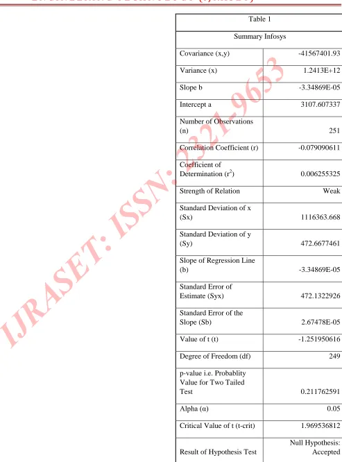
5. PERFORMANCE EVALUATIONS AND RESULTS
Table 1
Summary Infosys
Covariance (x,y) -41567401.93
Variance (x) 1.2413E+12
Slope b -3.34869E-05
Intercept a 3107.607337
Number of Observations
(n) 251
Correlation Coefficient (r) -0.079090611
Coefficient of
Determination (r2) 0.006255325
Strength of Relation Weak
Standard Deviation of x
(Sx) 1116363.668
Standard Deviation of y
(Sy) 472.6677461
Slope of Regression Line
(b) -3.34869E-05
Standard Error of
Estimate (Syx) 472.1322926
Standard Error of the
Slope (Sb) 2.67478E-05
Value of t (t) -1.251950616
Degree of Freedom (df) 249
p-value i.e. Probablity Value for Two Tailed
Table1. The study has chosen to perform analysis.
Figure 1.Sctter plot analysis Infosys.
6. CONCLUSION
The reason why there is no linear relationship between price and volume could be assigned to following[1,2] .
Risk appetite of most of the traders in stock market is varying ranging from low to high. This could be another reason why stock prices move faster when falling and thus not showing linear relation.
Prices and volume in the stock market is determined not only by fundamental factors like company’s performance and financial strength but also by speculative trading. This gives rise to unusual movement in price and volume both up and down.
Sometime there is divergence is price volume relationship. When rise in price is not supported by rise in volume, it is called divergence.
It is better to use prediction interval than confidence interval. Prediction interval will be suited for both delivery and intraday trading.
It is better to judge level of volume when market has started to have some practical significance of model.
7. FUTURE WORK
In future scope, improvement may be to modify the Findings of this study suggest that more can be learned from stock market about relation between trading volume and stock price. There may relation between these variables other than linear one.
REFERENCES
[1]Barbara Rockefeller. (2011). Drawing Trendlines. Technical Analysis For Dummies (2nd ed., pp. 169–182). Indianapolis: Wiley Publishin, Inc.
[2]Granger. C. W. J. & Morgenstem, O. (1963). Spectral Analysis of New York Stock Market Prices. Kyklos, vol. I6
[3]Osbome. M. F. M. (1959). Brownian Motion in the Stock Market. Operations Research, 1 (March-April 1959)
[4]Olaniyi, S. A. S., Adewole, K. S., & Jimoh, R. G. (2011). Stock Trend Prediction Using Regression Analysis – A Data Mining Approach. ARPN Journal of Systems and Software, 1(4), 154–157.
[5]Rinehart, M. (2003). Overview of Regression Trend Channel (RTC) (pp. 1–10).
[6]Ying. C. C. (1966). Stock Market Prices and Volumes of Sales. Ecommetrica, vol. 34, (http://www.jstor.org/discover/10.2307/1909776?uid=3738256 &uid=2&uid=4&sid=21104134756843)
[7] Altman, E.I. 1968. Financial ratios, discriminant analysis, and the prediction of corporate bankruptcy, Journal of Finance 23, 589-609.
[9]Bhattacharya, Hrishikes. 2007. Total Management by Ratios, 2nd ed., New Delhi, India: Sage Publications.
[10]Bildirici, Melike, and Özgür Ömer Ersin. 2009. Improving forecasts of GARCH family models with the artificial neural networks: An application to the daily returns in Istanbul Stock Exchange, Expert Systems with Applications 36(4), 7355-7362
[11]Connor, M.C. 1973. On the usefulness of financial ratios to investors in common stock, The Accounting Review, 339- 352.
[12]Chen, Mu-Yen. 2011 Predicting corporate financial distress based on integration of decision tree classification and logistic regression, Expert Systems with Applications 38(9), 11261-11272.
[13]Cheng, W; L. Wanger; and Ch. Lin. 1996. Forecasting the 30-year US treasury bond with a system of neural networks, Journal of Computational Intelligence in Finance 4, 10–6.
Davis, D. 2005. Business Research for Decision-Making, 1st ed., Belmont, CA: Thomson Brooks/Cole.
[14]Dutta, A., et al. 2008. Classification and Prediction of Stock Performance using Logistic Regression: An Empirical Examination from Indian Stock Market: Redefining Business Horizons: McMillan Advanced Research Series, 46-62.
[15] Guresen, Erkam, et al. 2011. Using artificial neural network models in stock market index prediction, Expert Systems with Applications 38 (8),10389-10397.