Compound Normal with Gamma Mixture Models A Model Characteristic Perspective

Technology (IJRASET)

Compound Normal with Gamma Mixture Models -

A Model Characteristic Perspective

Viziananda Row Sanapala1, Sreenivasa Rao Kraleti2, Srinivasa Rao Peri3 1

Associate Professor, Department of Computer Science & Systems Engineering, Andhra University, Visakhapatnam, India

2

Professor, Department of Statistics, Andhra University, Visakhapatnam, India

3

Professor, Department of Computer Science & Systems Engineering, Andhra University, Visakhapatnam, India

Abstract: In this paper, we discuss convergence performance issues of Compound Normal with Gamma Mixture(CNGM) and Truncated Compound Normal with Gamma Mixture(TCNGM) models that we have proposed in our earlier work in comparison to the normal mixture model(NM). We show that these models are feasible for mixture density estimation. Based on examination of coefficient of kurtosis, these models are shown to be preserving model characteristics of the more mesokurtic normal distribution and model better the leptokurtic deviations of normal distribution.

Keywords-- Probabilistic Framework, Compound Distributions, Truncated Distributions, Mixture Density Estimation, Expectation Maximization, MLE, NM, CNGM, TCNGM, EM, MAD

I. INTRODUCTION

In this paper, we address the issue of solving the more general problem of data clustering using mixture models that arise from within probabilistic framework. The main objective here is to look at two mixture models, the genesis for them being the finite normal mixture model, that we have proposed in our earlier work[1],[2]. The major issue addressed in this paper is to study the convergence performance of the two models in comparison to normal mixture model.

Physical considerations of the random experiment at hand can sometimes persuade one to consider modeling the experiment with a mixture. The experimenter may know that the phenomena that he is observing are a mixture; for example, the radioactive particle emissions under observation might be a mixture of the emissions of two, or several, different types of radioactive materials [3]. This paper is organized as follows. In Section II, we present an introductory treatment of probabilistic framework in general and in particular the issues related to the distribution models that have been considered for examination in our work. In Section III, we introduce the mixture density estimation problem, the maximum likelihood estimation approach, and the applications modeled as mixture density estimation problem.. In Section IV, we present the details that we have worked out in [1],[2].In Section V, convergence performance issues are discussed using a comparative approach. Finally we place our concluding remarks in Section VI.

II. PROBABILISTIC MODEL DRIVEN APPROACH

In probability and statistics, a probability distribution assigns a probability to each outcome of a random experiment. Based on the type of the random variable being discrete or continuous, the corresponding distributions are specified by probability mass functions or probability density functions. A parametric family of density functions is a collection of density functions that is indexed by a quantity called a parameter [3]. A probability distribution can either be univariate or multivariate. A univariate distribution gives the probabilities of a single random variable taking on various alternative values; a multivariate distribution is a joint probability distribution that gives the probabilities of a set of two or more random variables(dimensions) taking on combinations of values [3]. In the following subsections, we briefly discuss the underlying concepts related to our work.

A. Normal Distribution

A great many of the techniques used in applied statistics are based upon the normal distribution. A random variable X is defined to be normally distributed in the continuous domain if its density is given by[4]

( ) = ( ; , ) =

√

( ) ⁄ ₍₁₎

where the parameters ( ) ( ) satisfy −∞< <∞ and > 0. If random variable X is

Technology (IJRASET)

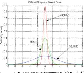
distribution, and is mesokurtic in nature identified by a bell shaped curve as shown in Fig. 1 (green in color). Platykurtic and leptokurtic variations of the same are shown in blue and red curves.

The above distribution has, as defined in [4], the following Pearson’s coefficients: Coefficient of skewness

= = 0 (2)

Coefficient of kurtosis

= = 3 (3)

Figure 1 Normal Densities X ~ N(μ,σ2)

B. Gamma Distribution

A random variable X is defined to be following gamma distribution if its density is given by

( ) = ( ; , ) =

Γ( )( ) (4)

where 0≤ <∞, > 0, > 0 . Here, r and are known as shape and rate(inverse of scale) parameters respectively. Γ(. ) is the gamma function. If r = 1, gamma density specializes to exponential density [3]. Figure 2 shows different shapes of gamma curves for = 1.

C. Compound Distributions

As stated by S. C. Gupta and V. K. Kapoor in [4], consider a random variable X, whose distribution depends on a single parameter θ which instead of being regarded as fixed constant, is also a random variable following a particular distribution. In this case, we say that the random variable X has a compound or composed distribution.

Figure 2 Gamma Densities (λ = 1)

D. Compound Normal With Gamma Distribution

As given in [5] by Normal L. Johnson et al, a compound normal with gamma distribution or ( , ) Λ ( ) is

Technology (IJRASET)

( ) = _{⁄ ( ⁄}

, ⁄ ) 1 +

( ) ( )⁄

(5)

where µ, c, and v are location, scale, and shape parameters. In the following sections, we will observe that that the above distribution models better the leptokurtic deviations of normal distribution.

The above distribution has the following characteristics whose derivations are detailed in[1], [2].

= (6) Second central moment about mean, i.e., variance is

= = _{( )} , ≥3 (7)

Third central moment about mean, is 0, since all odd moments about mean are zero. Fourth central moment about mean, is

=

( )( ) (8)

Pearson’s coefficients: Coefficient of skewness

= = 0 (9)

Coefficient of kurtosis

= = ( )

( ) (10) > 4 for finite kurtosis.

For different values of , this distribution has different shapes of frequency curves. As increases, tends to 3; thus, it includes mesokurtic distribution.

E. Truncated Distributions

In statistics, a truncated distribution is a conditional distribution that results from restricting the domain of some other probability distribution. Truncated distributions arise in practical statistics in cases where the ability to record, or even to know about, occurrences is limited to values which lie above or below a given threshold or within a specified range [3].

In general, if X is a random variable with density (. ) and cumulative distribution (. ), then the density of X truncated on the left at a and on the right at b is given by

( )

( ) ( ) (11)

For image segmentation problem, since the intensity values for gray level images usually range between 0 and 255, it is reasonable to model the data as a truncated distribution.

F. Truncated Compound Normal With Gamma Distribution

The probability density function of Truncated Compound Normal with Gamma Mixture(TCNGM) distribution after choosing left and right truncating points as a and b is defined by Equation(11) where

( ) = ⁄ _{( ⁄ , ⁄ )} 1 + ( )

( )

as defined in Equation(5), is the density function defined for the compound normal with

gamma distribution,

( ) = 1− , (12)

is the cumulative distribution function for some x taking value b such that ≥ , and

( ) = , (13)

is the cumulative distribution function for some x taking value a such that ≤ as derived in [2]. Here, , and ,

Technology (IJRASET)

distribution with a and b as left and right truncation point and is given as

( ) = _⁄

( ⁄ , ⁄ ) , , 1 + ( )

( )

(14)

where , , are incomplete beta functions. The ( ) in Equation (14) is the new density function for the

truncated compound normal with gamma distribution with a and b as left and right truncation points.

G. Mixture Distribution

A brief introduction as given by Mood et al in [3] to the concept of contagious distribution or a mixture is given here. If

(. ), (. ), … , (. ), … is a sequence of density functions which are either all discrete density functions or all probability density functions which may or may not depend on parameters, and , , … , , … is a sequence of parameters satisfying ≥0 and ∑∞ = 1_{, then ∑}∞ _{( ) is a density function, which is sometimes called contagious distribution or a mixture. Figure 3}

shows an example mixture distribution.

Figure 3 An Example Mixture Distribution

III. MIXTURE DENSITY ESTIMATION PROBLEM

Mixture density estimation problem is concerned with identifying local component distributions within the perspective of the global data distribution where the global data comprises a mixture of component distributions. This problem is generally solved using maximum likelihood approach which is explained below.

A. Maximum Likelihood Estimation Approach

In rough general terms, a maximum-likelihood estimate(MLE) of a parameter which determines a density function is a choice of the parameter which maximizes the induced density function (called in this context the likelihood function) of a given sample of observations. Maximum-likelihood estimation has been the approach to the mixture density estimation problem most widely considered in the literature since the use of high speed electronic computers became widespread in the 1960’s[6].

The customary way of finding a maximum-likelihood estimate is first to determine a system of equations called the likelihood equations which are satisfied by the maximum-likelihood estimate, and then to attempt to find the maximum-likelihood estimate by solving these likelihood equations. For mixture density problems, the likelihood equations are almost certain to be nonlinear and beyond hope of solution by analytic means. Consequently, one must resort to seeking an approximate solution via some iterative procedure like Expectation Maximization framework.

B. Maximum Likelihood Estimation Via Expectation Maximization

log-Technology (IJRASET)

likelihood found on the E step. Here, log-likelihood is considered since it is analytically simple form of the likelihood. These parameter-estimates are then used to determine the distribution of the latent variables in the next E step.

The EM algorithm for the mixture density estimation problem has been studied by many authors over the past several decades. It has been found in most instances to have the advantages of reliable global convergence, low cost per iteration, economy of storage and ease of programming, as well as a certain heuristic appeal. All in all, it is undeniably of considerable current interest, and it seems likely to play an important role in the mixture density estimation problem for some time to come.

C. Applications for Mixture Density Estimation Problem

The more general problem of data clustering may be considered as mixture density estimation problem. Big data analysis and data mining tasks use clustering as a kind of unsupervised learning for pattern analysis and machine learning. Image analysis is one such application of which image segmentation is one which may be addressed as mixture density estimation problem. The current literature on statistical image segmentation techniques mostly assumes the data describing the image as a mixture of component distributions, as shown in Fig. 3 [9],[10],[11],[12]. Segmentation methods use similarity property to detect distinct objects, each of which having similar properties for attributes like intensity value, texture, and others in a given image. In other words, the goal of image segmentation is to detect region homogeneity or similarity in the local neighborhood and extend this to the entire image based on different methods like thresholding, region growing, probabilistic distribution models, and other approaches.

IV. MAXIMUM LIKELIHOOD ESTIMATION USING CNGM AND TCNGM

In this section, we present the analytical expressions derived as in [1],[2] and their use during the construction of Expectation Maximization algorithm.

A. Analytical Expressions for Model Parameters

The probability density function of the CNGM model [8] is

( | ) = ∑ ( | ) (15) where the parameters are Θ= ( , … , , , … , ) such that = ( = ) with 0 < < 1 such that ∑ = 1. And each is probability density function parameterized by where = ( , , ). In other words, we assume we have M

component densities mixed together with M mixing coefficients or weights .

The probability density function , for a given component in compound normal with gamma mixture(CNGM) distribution , is defined, according to Equation (5), as

( | ) = ⁄ _{( ⁄}

, ⁄ ) 1 +

( ) ( )⁄

(16)

The analytical expressions for Θ= ( , … , , , … , ) for the above model are given in[1],[2] The solution in respect of Θ for CNGM is given as

= ∑ ( | ,Θ ) (17)

= ∑ | ,Θ (18)

= ( ) ∑ ( − ) ( | ,Θ ) (19)

=

∑ | ,Θ

−1 (20)

The probability density function , for a given component in truncated compound normal with gamma mixture(TCNGM) distribution , is defined, according to Equations (11), (12), (13), and (16) as

( | ) = _⁄

( ⁄ , ⁄ ) , , 1 + ( )

(21)

Technology (IJRASET)

=∑_∑ | ,Θ | ,Θ +

⁄ ⎣ ⎢ ⎢ ⎡ ⎦ ⎥ ⎥ ⎤

( ) , , , (22)

=( )∑_∑ ( ) | ,Θ | ,Θ +

⁄ ⎣ ⎢ ⎢ ⎡ ( ) ( ) ⎦ ⎥ ⎥ ⎤

, , , (23) =

, ,

, ,

∑ | ,Θ

∑ | ,Θ

− 1 (24)

and is same as that in Equation(17).

where x refers to each observation(individual pixel intensity value in the context of gray level images), , , and are, respectively, location, scale, and shape parameters of lth component of the mixture and (1 2⁄ , ⁄2) is the beta function.

B. EM Algorithm For The Proposed Models

In this subsection, we present the outline of EM algorithm [8] for the mixture model defined by compound normal with gamma mixture or its truncated form. The basic steps here are

Step1: Decide M, the number of segments based on the number of components of the mixture i.e., fix Θ= ( , … , , , … , ).

Step2: Initialize Θ.

Step3: Invoke EM algorithm.

EM Algorithm: /*Repeat E-step and M-step until convergence is reached*/ E-step: Compute the expectation as

( )_{( | ,}

Θ ) =

( ) | ( )

∑ ( ) | ( ) ( = 0,1,2, … )

where

( | ) is defined as in Equation(16) for CNGM and as in Equation (21) for TCNGM.

M-step: Compute update equations for

Θ= ( , … , , , … , ) using Equations (17),(18), (19), and (20) for CNGM and Equations (17),(22), (23), and (24) for TCNGM

( = 0,1,2, … )

The stopping criterion is

logℒ( )−logℒ( ) <

where ℒ is the likelihood of the parameter estimates, is error tolerance. In the above algorithm a and b, respectively, are set to 0 and 255 for our image segmentation experiment, since these values are considered as left and right truncation points for our TCNGM [1],[2].

C. Implementation And Results

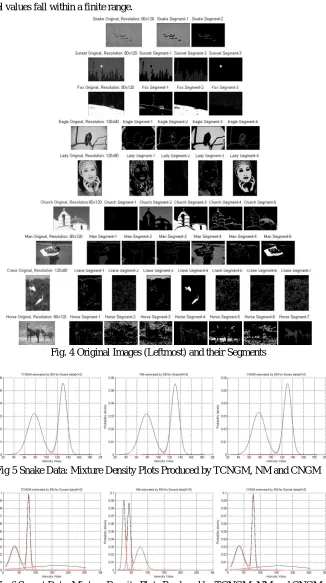
We have implemented the EM algorithm [8],[13] for the CNGM and its truncated version(TCNGM) in MATLAB and obtained fruitful segmentation results for those images as detailed in [1],[2].In our experiment, the initialization of the parameters for the specified number of clusters is done using K-means clustering. For those images considered for examination, we have obtained fruitful segmentation results as shown in Fig. 4 and their corresponding density plots in Figs. 5 through 13.

Technology (IJRASET)

compound normal with gamma mixture model.

The additional objective behind the proposed TCNGM model [2] is to study its feasibility to solve mixture density estimation problem in the context of truncated data distributions. We understand that image data distributions are well modeled as truncated distributions since the pixel values fall within a finite range.

Fig. 4 Original Images (Leftmost) and their Segments

Fig 5 Snake Data: Mixture Density Plots Produced by TCNGM, NM and CNGM

Technology (IJRASET)

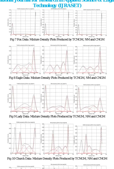
Fig 7 Fox Data: Mixture Density Plots Produced by TCNGM, NM and CNGM

Fig 8 Eagle Data: Mixture Density Plots Produced by TCNGM, NM and CNGM

Fig 9 Lady Data: Mixture Density Plots Produced by TCNGM, NM and CNGM

Fig 10 Church Data: Mixture Density Plots Produced by TCNGM, NM and CNGM

Technology (IJRASET)

Fig 12 Crane Data: Mixture Density Plots Produced by TCNGM, NM and CNGM

Fig 13 Horse Data: Mixture Density Plots Produced by TCNGM, NM and CNGM

V. CONVERGENCE PERFORMANCE ANALYSIS

In this section, convergence related issues for the models studied is presented since the three mixture models-TCNGM,CNGM, and NM exhibit different model characteristics and model complexities. In Subsection A, we present performance comparison for these models and in Subsection B, we present mean absolute difference inμ andσ between the classification data for all components and their maximum likelihood estimates as produced by the respective EM algorithms.

A. Convergence Performance Results

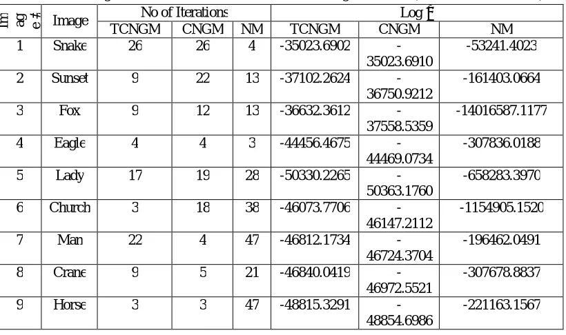
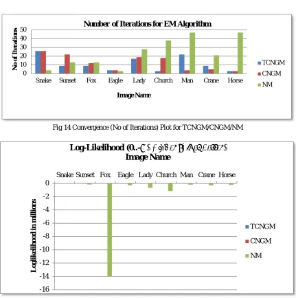
Convergence performance results in terms of number of iterations, log-likelihood, and segmentation time taken by the EM algorithm [8],[13] for the proposed truncated version of the compound normal with gamma mixture also appear to be good with respect to the other mixture models. Tables 1 and 2 show these results and the respective bar charts are shown in Figures 14, 15, and 16.

Table 1 Convergence Performance: No of Iterations and log-likelihood (TCNGM/CNGM/NM)

Im ag e # Image _TCNGM No of Iterations _{CNGM NM TCNGM CNGM} Log ℒ _NM

1 Snake 26 26 4 -35023.6902

-35023.6910

-53241.4023

2 Sunset 9 22 13 -37102.2624

-36750.9212

-161403.0664

3 Fox 9 12 13 -36632.3612

-37558.5359

-14016587.1177

4 Eagle 4 4 3 -44456.4675

-44469.0734

-307836.0188

5 Lady 17 19 28 -50330.2265

-50363.1760

-658283.3970

6 Church 3 18 38 -46073.7706

-46147.2112

-1154905.1520

7 Man 22 4 47 -46812.1734

-46724.3704

-196462.0491

8 Crane 9 5 21 -46840.0419

-46972.5521

-307678.8837

9 Horse 3 3 47 -48815.3291

-48854.6986

Technology (IJRASET)

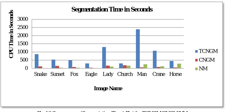
Table 2 Convergence Performance: Segmentation Time (TCNGM/CNGM/NM)

Im

a

g

e

#

Image Segmentation Time (Seconds)

TCNGM CNGM NM

1 Snake 866.3281 114.344 7.4063 2 Sunset 531.3750 145.609 35.2188 3 Fox 493.5469 79.5 34.4063 4 Eagle 295.3438 37.4688 10.5313 5 Lady 1300.641 166.063 99.6719 6 Church 300.8594 189.375 160.141 7 Man 2394.6094 58.3281 246.234 8 Crane 1079.5313 79.1094 127.953 9 Horse 450.7344 50.5781 283.969

Fig 14 Convergence (No of Iterations) Plot for TCNGM/CNGM/NM

Fig 15 Convergence (Log-Likelihood) Plot for TCNGM/CNGM/NM 0 10 20 30 40 50

Snake Sunset Fox Eagle Lady Church Man Crane Horse

N o o f It er at io n s Image Name

Number of Iterations for EM Algorithm

TCNGM CNGM NM -16 -14 -12 -10 -8 -6 -4 -2 0

Snake Sunset Fox Eagle Lady Church Man Crane Horse

Lo gl ik e li h o o d i n m il li o n s

Log-Likelihood (0..-

∞)(Higher values better)

Image Name

TCNGM

CNGM

Technology (IJRASET)

Fig 16 Convergence (Segmentation Time) Plot for TCNGM/CNGM/NM

The log-likelihood for TCNGM has been found to be very close to that of CNGM, since the genesis for the truncated version is the compound normal with gamma mixture, though there appears to be some significant difference in number of iterations. In respect of segmentation time, EM algorithm for TCNGM that is run, along with those for the other mixture models, on a PC with Pentium(R) 4 CPU 3.00 GHz, with 1GB RAM, has taken considerably more time than the others for all the images considered for experimentation. The reason for this, unlike CNGM, might be due to the additional terms in the update equations that incurred substantial computational overheads. Time complexity for running EM algorithm, in general, is said to be quadratic in nature [6], though it can be more in certain formulations. Since we have used segmentation time as an alternative specification, the run time complexity study is not addressed in this work.

B. Mean Absolute Difference In μ And σ

In this section, we present an additional study that has been carried out in [2] to examine the deviations of the observed segmentation data from the corresponding maximum likelihood estimates for the parameters, as computed by the compound normal with gamma mixture model, its truncated version, and the normal mixture model. Average absolute difference in mean (μ) and

standard deviation (σ) between the said observed data and the corresponding estimates are considered for this purpose. The mean

absolute difference in μ and σ for the image data are defined below, which have been computed based on the given number of respective image segment distributions for each image data.

= ∑ − (25)

= ∑ − (26)

In the Equations (25) and (26), and , respectively, stand for mean absolute difference in μ and σ. For each segment i ,

ranging between 1 to K , and are mean and standard deviation observed and and are the corresponding maximum likelihood estimates. The maximum likelihood estimate for σ in respect of the compound normal with gamma distribution and its

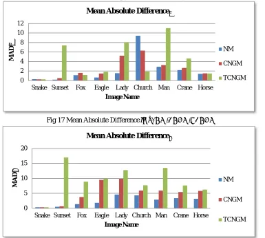
truncated version is computed using Equation (7), which defines the variance ( ) as a function of scale(c) and shape(v) parameters. The results obtained for and in respect of normal mixture, compound normal with gamma mixture and its truncated version are presented as bar charts in Figs. 17 and 18. A keen observation at the figures suggest that all the three models are subject to deviations in one or the other measure across the images considered for examination. The reason for this might be due to the influence of overlapping densities across component distributions in the mixtures [1],[2]. This statement is supported by the respective density plots shown in Figures 5 through 13.

0 500 1000 1500 2000 2500 3000

Snake Sunset Fox Eagle Lady Church Man Crane Horse

C P U Ti m e i n S e c o n d s Image Name

Segmentation Time in Seconds

TCNGM

CNGM

Technology (IJRASET)

Fig 17 Mean Absolute Differencein μ: NM/CNGM/TCNGM

Fig 18 Mean Absolute Differencein σ: NM/CNGM/TCNGM

VI. CONCLUSIONS

In this paper, the EM algorithm for the models studied in [1],[2] has been constructed and it is implemented using MATLAB. This has been applied to solve image segmentation problem as a mixture density estimation problem. Here, we have re run the implementation in [1] for normal, compound normal with gamma mixture model to check for consistency in the results between runs and used these results to compare with those obtained for the truncated version presented in [2] of the compound normal with gamma mixture model. Convergence performance of the EM algorithm for the proposed model in terms of number of iterations, log-likelihood, and segmentation time in comparison with that for normal and compound normal with gamma mixture models has been thoroughly examined. In addition to this, deviations of the observed segmentation data from the respective maximum likelihood estimates for the models in terms of average absolute difference in mean(μ) and standard deviation(σ) are

reported.

VII. ACKNOWLEDGMENT

The authors thank Andhra University, Visakhapatnam, India, where they have put up more than twenty five years of teaching service, for the support they have received from time to time.

REFERENCES

[1] Viziananda Row Sanapala, Sreenivasa Rao Kraleti, and Srinivasa Rao Peri. Image Segmentation Using Compound Normal with Gamma Mixture Model,

International Journal of Computer Science Issues, Volume 12, Issue 4, July 2015, ISSN (Print): 1694-0814 | ISSN (Online): 1694-0784, www.IJCSI.org.

[2] S. Viziananda Row, Image Segmentation Using Compound Normal with Gamma Mixture Model and its Truncated Version, Ph. D. Thesis, Andhra University,

Visakhapatnam, India, 2016.

[3] Alexander M. Mood, Franklin A. Graybill, and Duane C. Boes. Introduction to the theory of Statistics, Tata McGraw-Hill,Third Edition, 2001.

[4] S. C. Gupta and V. K. Kapoor. Fundamentals of Mathematical Statistics, Sultan Chand and Sons, New Delhi, Eleventh Edition, 2002.

[5] Normal L. Johnson, Samuel Kotz and N. Balakrishnan. Continuous Univariate Distributions,Vol-I , Second Edition. John Wiley&Sons, 2007.

0 2 4 6 8 10 12

Snake Sunset Fox Eagle Lady Church Man Crane Horse

M

A

D

μ

Image Name

Mean Absolute Difference_μ

NM CNGM TCNGM 0 5 10 15 20

Snake Sunset Fox Eagle Lady Church Man Crane Horse

M

A

D

σ

Image Name

Mean Absolute Difference_σ

NM

CNGM

Technology (IJRASET)

[6] Richard A. Rednerf and Homer F. Walker. Mixture Densities, Maximum Likelihood and the EM Algorithm, SIAM Review, vol. 26, no. 2, pp 195-239 April

1984.

[7] A. P. Dempster, N. M. Laird and D. B. Rubin. Maximum-likelihood from incomplete data via the EM algorithm, J. Royal Statist. Soc. Ser. B

(methodological), 39 (1977), pp. 1-38.

[8] J. A. Bilmes. “A gentle tutorial of the EM algorithm and its application to parameter estimation for Gaussian mixture and hidden Markov models.” International

Computer Science Institute, Berkely CA, 94704, pp 1-13.

[9] T. Lei and J. K. Udupa. Performance evaluation of finite normal mixture model-based image segmentaion techniques. IEEE Transactions on Image Processing,

vol 12, no 10, pp. 1153-1169, 2003.

[10] J. Zhang and J. M. Modestino. A model fitting approach to cluster validity with application to stochastic model based image segmentation, IEEE Transactions

on Pattern Analysis and Machine Intelligence, vol. 12, no. 10, pp.1009–1016, 1990.

[11] T. Lei and W. Sewchand. Statistical approach to x-ray CT imaging and its applications in image analysis—Part 2: A new stochastic model based image

segmentation technique for CT image, IEEE Transactions on Medical Imaging, vol. 11, no. 1, pp. 62–69, 1992.

[12] Z. Liang and J. R. MacFall. “Parameter estimation and tissue segmentation of multispectral MR images.” IEEE Transactions on Medical Imaging, vol. 13,

no.3, pp. 441–449, 1994.