2016 International Conference on Computer, Mechatronics and Electronic Engineering (CMEE 2016) ISBN: 978-1-60595-406-6
Vehicle Automation-Algorithm for Changing/Merging Lane Behavior
Yao CHEN
1,*, Yan-long JIANG
2and Philippe GICQUEL
31,2
Nanjing University of aeronautics and Astronautics (NUAA), China 3
Customer In the Loop for System engineering (CIL4Sys), France
*Corresponding author
Keywords: Intelligent vehicle, Changing/merging lane, Obstacle avoidance, Web simulation,
Function development.
Abstract. The object of this article is to improve the intelligent vehicles' "ACC system" (Adaptive Cruise Control) and "Braking system" function and permits the vehicle have more sophisticated changing lane behavior and be able to deal with more complex situations when changing lane. Then test the function in the web simulator, which is designed by a start-up called CIL4Sys and is software whose robustness for different functions needs to be test.
Firstly, to improve the vehicle's changing/merging lane behavior, two algorithms are created:
Algorithm 1 "changing/merging lane decision algorithm" sub system and Algorithm 2 "obstacle avoidance algorithm" sub system. The combination of these two algorithms serves as two different functions. A function dealing with the full process of intelligent vehicle's changing/merging lane in highway: Function 1 "Changing/merging lane function". And a function for obstacle avoidance in city road: Function 2 "Obstacle avoidance function". The main tools for developing the algorithm is Matlab / Simulink, the main environment for compiling the algorithm is VS2012.
To test the function, a UML model is needed to integrate the function to the profile of that of the enterprise. And the UML model for this sub system has been constructed using PTC Integrity Modeler. Please note that all these functions consider the traffic act.
Introduction
The idea of a vehicle full automation is, among others, motivated by the necessity of increasing the capacity of the highways without reducing the security of the passengers.
There exist already a lot of assistance driving system such as CC (Cruise Control), ACC (Adaptive Cruise Control), Stop & Go, AACC (a combination of the function of the high-speed ACC and low-speed SG), CACC (Cooperative Adaptive Cruise Control), ADAS (Advanced Driver Assistance Systems) [1,2]. These kind of systems can help drivers have more comfortable driving experience or more keep safe during driving. But that is not enough for intelligent vehicles. The ITS (Intelligent Transport System) is independent on humans and it has not only the system which helps control the vehicle but also the redundancy design. ITS has its own ECU to detect errors and error correcting system which can help the vehicle out of danger [3].
In addition, traffic accidents which happens during the process of changing lane is by no means rare and the consequence is disastrous, especially when this vehicle is on multiple lanes [4]. To increasing the safety and the efficiency of road, it is necessary to conduct a research on vehicles' changing lane. In addition, the highly development of the measure technologies makes automatic changing lane possible.
thus increase its efficiency and also eliminate traffic jams and traffic accidents both in highway and in city road.
Vehicles change lane in order to continue the journey. Then lane changing provides a maneuver for a fast vehicle to pass a slow vehicle, which can be observed everywhere on the highway. Lane changing decisions in driving situations including the influence of traffic signals, obstructions and different vehicle types such as heavy vehicles and dissatisfaction of driving conditions. Vehicle lateral control is a challenging problem in areas of ITS and automatic control for autonomous vehicles [5]. Collision avoidance is one of the most important issue in lane changing and lateral control. Lane changing/merging collisions are responsible for one tenth of all crash-caused traffic delays often resulting in congestion.
The researched of the above problems is based on trajectory planning. [6] Firstly presents a set of paths called bi-elementary paths, which are smooth and feasible for a car-like robot. That means their tangent direction is continuous and they respect a minimum turning radius constraint and they can be followed by a real vehicle without stopping. After that, a lot of methods for predicting vehicle's trajectory have been developed. These methods can be divided into three major types: (1) Acceleration-based trajectory planning; (2) Polynomials-based trajectory planning; (3) Sate-Space representation trajectory planning. [7] Using four different methods to design the virtual desired trajectory (VDT): (a) Circular trajectory; (b) Cosine trajectory; (c) 5th order polynomial trajectory; (d) Trapezoidal acceleration trajectory. The author's objective is to using these VDTs to predict the time for changing thus guaranteeing the passengers' comfortable, that is to say, the lateral acceleration limit and the lateral jerk limit are taken as 0.05 g and 0.1 g/s, respectively. [8] Assuming the acceleration in lateral direction as piece wise function using trigonometric functions Eq. 1:
ifNot a gingLane duringChan t t y t y direction a Duration overtaking t Gap overtaking y y e e e e y e e , 0 , 2 sin 2 (1) [9] Using polynomial function to plan the trajectory and calculate the trajectory which is obstacle avoidance. The algorithm is based on the use of polynomials for trajectory planning and the use of simplified s-topes for obstacle representation. Dynamic constraints are also taken into account. The resulting criterion for the selection of the desired and achievable trajectory involves the selection of a single coefficient. Illustrative examples show the main advantages of the algorithm especially in the case of lane changing with multiple obstacles. [10] Assuming the acceleration in lateral direction as piece wise function using polynomial functions. So, it is similar as a sinus function. [2] describes the trajectory for changing lane as two simple equations using trigonometric function respectively in the longitudinal and lateral direction. [11] uses the state-space representation to model the system, this model considered also the radius of the road. The Acceleration-based model takes into account the cinematic characteristics while the Polynomials-based model uses the mathematical fitted method. In this article, these two methods have been used. The former is usable for calculating commands for vehicles and the latter is very useful for obstacle-avoidance.
Realization of the Object
Highway: Changing/Merging Lane Function
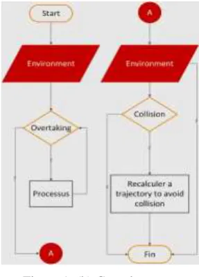
velocity in "ACC". Normally, the vehicle will be blocked by the front vehicle, this will reduce the efficient of the road. The problem can be solved by adding a "Changing/merging lane decision function": the vehicle has more opportunity to arrive the preset velocity if it can change lanes deftly. Also, the "Obstacle Avoidance algorithm" serves as a redundant design for the Changing/merging lane function. Figure 1 (a) shows the process of "changing/merging lane decision algorithm". The algorithm starts with analyzing the environment, which includes the road information, the behavior of the other road users, traffic act and safety constraints. Then makes a decision for changing/merging lane: if "decision = true" the system goes to changing/merging lane process, otherwise return to "start". Obviously, for intelligent vehicles, we should not only just make the decision to tell the vehicle if it can change lane, but also help the vehicle to finish the changing lane mission. That means we should provide a solution in emergency cases. For example, the vehicle receive the command to change lane, but another vehicle arrives rapidly or the cinematic parameters of the others vehicle changes a lot during its mission, which may cause problems for the ego vehicle (collision). In such occasion, it is necessary to provide the vehicle a trajectory which can avoid the collision or tells the vehicle to brake. Figure 1 (b) presents the complete system for this function: after the decision algorithm gives a positive decision, the ego vehicle begins to changing/merging lane, and the "obstacle avoidance algorithm" has been launched at the same time. Thus, the "obstacle avoidance algorithm" can provides the ego vehicle a no collision trajectory in case of emergency.
Figure 1. (a) Simple system Figure 1. (b) Complete system.
If there exists not any safe trajectory, the braking system will be launched, which is integrated into the obstacle avoidance sub system. In the case of existing safe trajectory, a controller should be used. But this is not presented in this article.
Please note that the "changing/merging lane decision algorithm" is used and only used in "changing/merging lane function". And it only works before the ego vehicle begins to changing/merging lane and keeps dormant after giving a positive decision. In this function, the "obstacle avoidance algorithm" is used to deal with the case when the ego vehicle receives the positive decision for changing/merging lane and meets the danger of collision. It begins working as soon as the process of changing/merging lane begins.
City-Road: Obstacle Avoidance Function. In the case of city road, the "obstacle avoidance function" is used to deal with the case when the ego vehicle is running on the city road and when emergency comes. If the ego vehicle cannot avoid collision with just a simple "Emergency braking system", the "obstacle avoidance function" will be invoked.
[image:3.595.355.499.339.539.2]Avoidance" sub system and test. (3) Testing the function in CIL4Sys's web simulator to observe its performance.
PART I: Changing/merging lane decision algorithm
Trajectory planning method. In this article, Eq. 1 is used in the last step of decision to predict/estimate collision because this method mostly obeys the dynamic principle. That is to say the acceleration based model. Furthermore, the total velocity is assumed to change with the acceleration of ame. For considering the radius of the road, a part of centrifugal acceleration has been added to the lateral direction for each vehicle. The acceleration in each direction can be calculated easily Eq. 2:
2 2
2
, 0
,
total total total
total total
y x
me total
l centrifuga y
l centrifuga y
y
road total l centrifuga
a a a
a a
ifNot a
a
gingLane duringChan
a a a
r v a
(2)
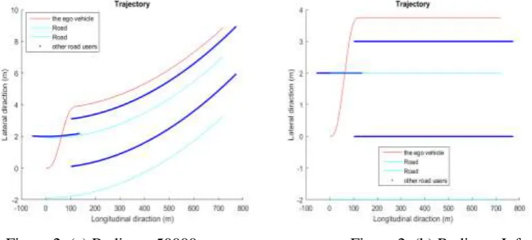
Hence, the velocity in each direction can be calculate by integrating their acceleration in each direction and the travel distance can also be calculated by integrating their velocity in each direction. So the velocity and the coordinate of each vehicle can be predicted. This method is used for the 4th level of decision (4 level in total). The figures as follows presents the trajectories when the ego vehicle runs in the road straight and when it runs in the road with a radius of 50000m.
Figure 2. (a) Radius = 50000. Figure 2. (b) Radius = Inf.
[image:4.595.106.491.480.654.2]
others s
s
others me
e e s
me others
V t d
d V
V t t d
safetyTime t
S S
d
0 0
(3) Note that the d
0 is the initial distance between vehicles before changing lane and the d
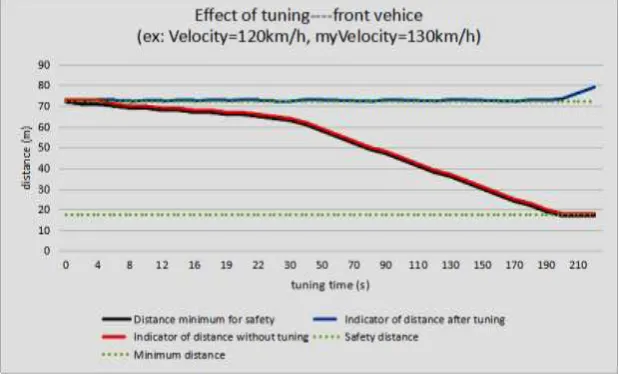
te is that of vehicles after changing lane. [image:5.595.143.453.249.436.2]Modify the Safety Distance by Adding Tuning Time. Because in some situations, the distance between the ego vehicle and other vehicle grows over time. So there exists the cases that the vehicles which is defined dangerous become no longer dangerous after just a little period of time. It is meaningful to add a "tuning time": the effect of adding tuning time equals that we reduce the safety time.
Figure 3. Effect of tuning time.
Take the case of vehicle in the target lane for an example: It means when the ego vehicle finishes changing lane, the distance between the ego vehicle and the other vehicle is less than tsVvehicleRear, but increase to this value after the tuning time. In addition, we should also guarantee the distance between the two vehicles after changing lane is more than five times of the vehicle in front. This can augment the probability for changing lane and augment the traffic flow. However, we should pay attention for the cases who can't use tuning time: the distance between the ego vehicle and the other vehicle reduces over time. Take the vehicle left rear in the case that the ego vehicle wants to turning left as an example Eq. 4, and the effect of tuning time is presented as follows Figure 3.
As you can see, the indicator of distance augment after adding tuning time. And the safety constraints is "indicator of distance > safety distance", that is to say, it is easier for the vehicle to attain the safety constraints.
t t t
V V
d 0d
tuningTime t
others me
e
e
(4) Process of Decision. The process of decision is divided into 4 levels: pre-decision; Analyze the road users which are also in the process of changing/merging lane; judge their safety distances; predicting collision. The higher the level is, the harder to achieve.
After all these preparations, the process of decision is divided into 4 principle sections increasing level: Analyze the road users which are also in the process of changing/merging lane; Calculate the distance between the ego vehicle and all the other vehicles to see whether it is sufficient safe; Predict if there exits collision using the "acceleration based trajectory planning" method; Calculate the time limit for beginning changing lane which can guarantee the safety of vehicle. But the fourth part hasn't been used in the final model.
Conclusion of the Model. The decision model considers: (1) the acceleration of the ego vehicle varies with consignment, (2) the acceleration of the other road users is fixed as a constant value which corresponds with their initial acceleration, (3) the lateral and longitude speed limit, the lateral and longitude acceleration limit, (4) the radius of the road, (5) the distance minimum with each types of the vehicles are calculated more accurate which includes the effects of the road radius, acceleration, tuning time and etc. (6) The effect of running time which lightly dampens the security but elevate the efficiency for the vehicle's changing/merging lane. (7) The effect of the position deviation of the ego vehicle.
PART II: Obstacle Avoidance Algorithm
Trajectory Planning Model. The main idea to do the part "Obstacle Avoidance" from [9]. This method uses two vectors: The vector X and the vector Y to present the initial states and the final states:
coordinatexinitial velocityxinitial accelerationxinitial coordinateyinitial velocityyinitial accelerationyinitial
X ; ; ; ; ;
coordinatexfinal velocityxfinal accelerationxfinal coordinateyfinal velocityyfinal accelerationyfinal
Y ; ; ; ; ;
The output of this method is the angle command and the acceleration command.
Given the initial and final state of the ego vehicle, the initial state of the obstacles and a preset duration for finishing obstacle avoidance, we can provide a group of possible trajectories. These trajectories will be selected by angle constraints, acceleration constraints and velocity constraints. Finally, the system provides the ego vehicle an angle, an acceleration and the indicator for obstacle avoidance, which is "true" when obstacle avoidance sub system is launched and vice versa. This algorithm will be invoked each 40 ms until the ego vehicle find a safe position.
The trajectory is presented by a group of polynomials, one polynomial for the longitude direction and the other for the lateral direction. In the case without obstacle, the polynomials for both two directions are "quintic polynomials". In the case with obstacle(s), one order is added to the polynomial of the longitude direction Eq. 5 for considering the obstacles and provides the trajectory with the capacity of obstacle avoidance.
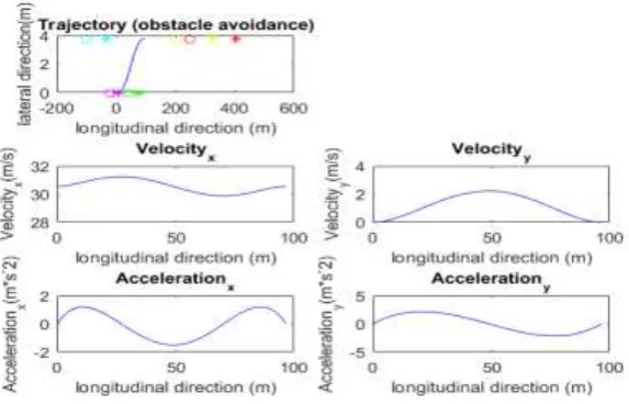
0Figure 4. Dynamic parameters.
An example is presented. In this case the inputs of the system are: the initial position of the road user No.1 which is presented as
coordinatex,coordinatey
moves from (250, 3.75) to (425, 3.75). The same method for presenting the other road users; road user No.2: (-100, 3.75) to (-25, 3.75); road user No.3: (-20, 0) to (10, 0); road user No.4: (200, 3.75) to (340, 3.75); road user No.5: (40, 0) to (80, 0); duration = 3.6 second; initial state of the ego vehicle = [0; 30.5556; 0; 0; 0; 0]; the test tells that the vehicle can't avoid collision using braking.As you can see, the "vehicle front" and the "vehicle rear" are all very close to the ego vehicle and the velocity of the "vehicle rear" is large, the velocity of the "vehicle front" is very small. It is necessary to do obstacle avoidance. The test results prove that the obstacle avoidance part can always find a solution when the distance between the ego vehicle and the "front vehicle" is larger than 40m and with velocity equals to 0 m/s. The dynamic parameters in the coordinate system of the road is presented in Figure 4.
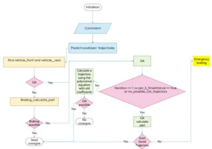
Figure 5. Diagram for obstacle avoidance function.
Please note that the "OA" in the figure means "Obstacle Avoidance". The ego vehicle begins with the normal braking part, whose acceleration is an inverse bell curve, then begins to do obstacle avoidance if necessary. If these above two part cannot avoid the other vehicle or make the ego vehicle safe, a constant acceleration with the value of -8 m*s^-2 is applied, called the urgency braking part.
Also, as you can see, the "Obstacle avoidance algorithm/function" is used both in highway as redundant design for "Changing/merging lane function" and in city road as emergency measures. But the strategy changed. In highway, the ego vehicle cannot brakes until velocity reaches null, so the ego vehicle prefers at first finding a new no-collision trajectory then brakes if it is necessary. In city road, the ego vehicle doesn't want a complicated trajectory but prefers at first braking. If the ego vehicle cannot avoid collision by braking, it begins to find a no-collision trajectory. This is why another output "OA" is added into the model.
This function should be invoked each 40 ms, that is to say, there exist a lot of exceptions. Doing test is very important. Also, because it takes a lot of time to calculate a trajectory for obstacle avoidance, a lot of improvements have been added to make the algorithm more efficiency, please see my report for more details.
PART III: Test of the Two Functions
Results. There presents the results from two cases of simulation.
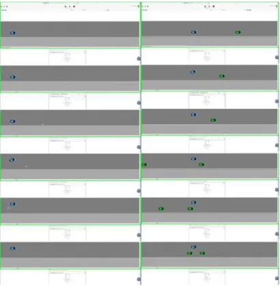
Figure 6. (a) Obstacle avoidance in the case of pedestrian. (b) Obstacle avoidance in the case of vehicle.
The first one is the case when there is a pedestrian Figure 6 (a). The ego vehicle launches the sub system obstacle avoidance to keep both of them safe. The vehicle begins with deceleration then launch the obstacle avoidance part it finds a pedestrian nearby is crossing the road and the distance is smaller than the minimum distance. The vehicle finishes changing lane in a short period of time (which changes according to situation) and then return to relatively stable state. The second one is the case when there is a vehicle stopped in front of the ego vehicle and, in the same time, there exists a rear vehicle which rolls very fast Figure 6 (b). Hence, the ego vehicle launches the obstacle avoidance to avoid accident. The vehicle begins with obstacle avoidance part to avoid hurting the front vehicle and to avoid being hurt by the fast rear vehicle.
Conclusion
[image:9.595.93.504.109.532.2]a part of the future work. From which, the traffic flow of the route can be controlled more and more adequate and the efficiency of the utilization of the road may be greatly improved.
References
[1] Malinauskas R. The Intelligent Driver Model: Analysis and Application to Adaptive Cruise Control[J]. 2014.
[2] Petrov P, Nashashibi F. Adaptive steering control for autonomous lane change maneuver[C]//Intelligent Vehicles Symposium (IV), 2013 IEEE. IEEE, 2013: 835-840.
[3] The difference between its and adas (in chinese), https://www. zhihu.com/question/36884389.
[4] Van Dijck T, van der Heijden G A J. VisionSense: an advanced lateral collision warning system[C]//IEEE Proceedings. Intelligent Vehicles Symposium, 2005. IEEE, 2005: 296-301.
[5] Khodayari A, Ghaffari A, Ameli S, et al. A historical review on lateral and longitudinal control of autonomous vehicle motions[C]//2010 International Conference on Mechanical and Electrical Technology. 2010.
[6] Scheuer A, Fraichard T. Collision-free and continuous-curvature path planning for car-like robots[C]//Robotics and Automation, 1997. Proceedings, 1997 IEEE International Conference on. IEEE, 1997, 1: 867-873.
[7] Chee W, Tomizuka M. Vehicle lane change maneuver in automated highway systems[J]. California Partners for Advanced Transit and Highways (PATH), 1994.
[8] Jula H, Kosmatopoulos E B, Ioannou P A. Collision avoidance analysis for lane changing and merging[J]. IEEE Transactions on vehicular technology, 2000, 49(6): 2295-2308.
zhihu.com/question/36884389.
[9] Papadimitriou I, Tomizuka M. Fast lane changing computations using polynomials[C]//American Control Conference, 2003. Proceedings of the 2003. IEEE, 2003, 1: 48-53.
[10] Feng J, Ruan J, Li Y. Study on intelligent vehicle lane change path planning and control simulation[C]//2006 IEEE International Conference on Information Acquisition. IEEE, 2006: 683-688.
[11] Eidehall A, Petersson L. Statistical threat assessment for general road scenes using Monte Carlo sampling[J]. IEEE Transactions on intelligent transportation systems, 2008, 9(1): 137-147.