2016 International Conference on Artificial Intelligence and Computer Science (AICS 2016) ISBN: 978-1-60595-411-0
An Improved ML-kNN Algorithm by Fusing Nearest
Neighbor Classification
Yong ZENG, Hao-ming FU, Yu-ping ZHANG and Xi-ya ZHAO
School of Automation Engineering, University of Electronic Science and Technology of China, Chengdu 611731, China
Keywords: Multi-label Classification, ML- kNN, IML- kNN, Nearest neighbor weighted.
Abstract. Based on the ML-kNN multi-label classification algorithm of probability and statistics, the
k neighbors of unclassified sample are implicitly deemed that they have the same effect on classification result while ignoring the influence of the distances between k neighbors and unclassified sample. This paper proposes an improved ML-kNN algorithm by fusing nearest neighbor classification: IML-kNN. On the basis of the traditional ML-kNN algorithm, the algorithm considers the influence of the nearest neighbor and k neighbors of unclassified sample. Numerical simulation results show that the IML-kNN algorithm can have a good classification effect on the multi-label evaluation metrics.
Introduction
Research on multi-label classification problems has become the focus of many scholars, because it is widely presented in the current era of big data. For example, in the film category, a film may belong to a number of predefined themes, such as "action movie" and "comedy"; in functional genomics problem[1, 2] each gene may have a variety of features such as "protein synthesis" and "transcription";
and it is also applied to text classification [3-5], video semantic annotation [6], image classification and
other fields. Multi-label problems in mathematical language can be described as: definition of d-dimensional input space of sample x , and definition of a limited set of labels y={β1,β2,...,βq}, the
classification question is giving a training data set T={(x1,Y1),(x2,Y2),...,(xm,Ym)}(xi∈Rd,Yi∈y), to work
out a multi-label classifier h:Rd→2y, and h can optimize some of the specified assessment criteria. In
practice, a real-valued mapping function f: Rd×y→R is usually figured out on the solution process.
Assuming that a given instance and its associated set of labels, a good classifier will produce a greater value for selected labels, while a smaller value for non-selected labels, namely
f(xi,y1)>f(xi,y2)(y1∈Yi,y2∉Yi).
There are two main methods to solve the multi-label classification problem: problem transformation method and algorithm transformation method. Multi-label classification problem is converted to binary problem, label sorting problem for problem transformation method. Representation algorithm are BR [7, 8] (binary relevance) and LP [9] (label power set).
Algorithm transformation method adjusts existing single-label classification algorithm to deal with multi-classification problem. AdaBoost.MH [10] is extended from the AdaBoost algorithm to
determine label set by minimizing the Hamming loss. SVM-based Rank-SVM [11] constructs a SVM
classifier for each category marker. This method takes into account correlation and irrelevant markings of each sample by using ranking loss. The objective optimization problem can be transformed into a quadratic programming problem, but the training is very time consuming. The ML-kNN [12] based on classic kNN algorithm considers label selection information of the k nearest
neighbors (kNN) of one sample, and uses the maximum a posteriori probability criterion (MAP) to predict classification information of samples to be classified. This method is simple and effective, but the relevant information of label combinations is not considered. To this end, a new multi-label lazy learning algorithm [13] IMLLA is proposed in [14] by fully investigating the correlation between
labels. In literature [15], a multi-label classification algorithm based on Naive Bayes (MLNB) is designed and a feature selection mechanism is added at the same time. In this paper, we propose a new improved algorithm based on ML-kNN: considering the influence of the nearest neighbor and k
neighbors of unclassified sample, and this effect is quantified by the weighted value. Finally, the ML-kNN algorithm and IMLLA algorithm are compared with the improved algorithm on the test set.
ML-kNN Algorithm
The ML-kNN algorithm takes advantage of the maximum a posteriori probability criterion, which can convert the conditional parameter probabilities to get a classification function, which combines with kNN.
For each test instance x, ML-kNN firstly identifies its kNNs N(x) in the training set. Let H1l be the
event that x has label l, while H0l be the event that x has not label l. ElCx(l)denotes the event that,
among the kNNs of x, there are exactly Cx(l) instances which have label l, where Cx(l) counts the
number of neighbors of x belonging to the lth class. For each label, the probability of P(Hbl) and
P( ElCx(l)|Hbl) are obtained by counting the corresponding frequencies of labels in the training data set
as certain rules.
Improved ML-kNN algorithm: IML-kNN
For each sample in the data set, its k neighbors' label set is largely similar with the sample' label set. Its similarity will change with the distance between neighbors and the sample. The distance is inversely proportional to the similarity. Normally, as the distance gets farther, the similarity gets smaller and vice versa. Based on this, we consider the influence of unclassified sample’s k neighbors and the nearest neighbor simultaneously, and this effect is quantified by the weighted value, resulting in getting a new weighting function classification:
Nx(l) represents the value of label l among the nearest neighbor of a sample x, value is 0 or 1 for
binary classification.1/k and (k-1)/k denote weighting coefficients, in this paper, the influence on the label set of the sample from its k nearest neighbors’ label set is considered equal, so the weighting coefficient of the nearest neighbor sample is 1 / k, and (k-1) / k for the k neighbors. Then we will discuss the effect of the k values on the classification accuracy. The algorithm steps are as follows.
Algorithm 1 Improved IML-kNN algorithm pseudo-code description Input: training set T, the unknown sample t
Output: label set of the unknown sample t
Step 1: Calculating the priori probability of each label l∈y
Step 2: Calculating the sample xi (i=1,2,...m)’s k neighbors N(xi)
Step 3: Calculating the posterior probability of each label l∈y
) 2 ( )). ( ) ( 1 -) ( 1 ( max arg )
( {01} ()
∈ l b l l C l b x , b
x k P H P E |H
k l N k l
y = × + × x
im l l
x
l s y l / s m P H P H
H
P( 1) ( 1 i( )) ( 2 ); ( 0) 1 ( 1);
p c K s / j c s |H E P p c K s / j c s |H E P do ,...,k , for j c e c
els c then c l y if y l C do ,...,m , for i j c j c do ,...,k , for j
y do for l k p ' ' l l j k p l l j ' ' x x N a a x ' i i i ); ] [ ) 1 ( ( ]) [ ( ) ( ); ] [ ) 1 ( ( ]) [ ( ) ( } 1 0 { ∈ ; 1 ] ∂ [ ] ∂ [ ; 1 ] ∂ [ ] ∂ [ ) 1 ) ( ( ) ( ∂ } 2 1 { ∈ ; 0 ] [ ; 0 ] [ } 1 0 { ∈ ∈ ∑ ∑ ∑ 0 0 0 1 ) ( ∈ = = + + × + = + + × + = + = + = == = = = = (1) ). ) ( max arg ) ( max arg )
( {01} ( )
∈ ) ( } 1 0 {
∈ P H |E P H P(E |H l y l b l l C l b , b l l C l b , b
x = x = x
Step4: Calculating the k neighbors of the unknown sample t Step 5: Calculating the unknown sample t’s labels value yt(l)
As shown in algorithm 1, calculating prior probability vector and conditional posterior probability vectors (where s = 1, generating Laplace filter) for each label by using the ML-kNN in the training data set, then on the test data set for each unknown sample t, calculating the total neighbor number whose label is selected from the sample t’s k neighbors. At last, we classify the sample t by using the improved classifier function (equation (2)).
Experimental Results and Analysis Experiment settings
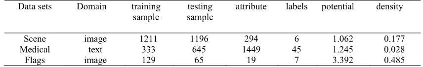
[image:3.612.91.519.364.432.2]Details of the three data sets are shown in Table 1. The label potential is average number of labels selected in one sample, labels density is the ratio of the potential with total number of labels.
Table 1. baseline data set.
Evaluation Indicators
(1) Hamming loss: evaluates how many times an instance-label pair is misclassified, i.e. a label not belonging to the instance is predicted or a label belonging to the instance is not predicted.
Where Q is the number of labels set, h(xi) is the classification result, h(xi)ΔYi stands for the
symmetric difference between the actual labels set of sample and classification result.
(2) Coverage: evaluates how far we need, on the average, to go down the list of labels in order to cover all the proper labels of the instance.
(3) One-error: evaluates how many times the top-ranked label is not in the set of proper labels of the instance.
The most foremost label on the result labels set is selected on the actual labels set, H(xi) =1,
otherwise H(xi) = 0.
(4) Ranking loss: evaluates the average fraction of label pairs that are reversely ordered for the instance.
Data sets Domain training
sample sample testing attribute labels potential density
Scene image 1211 1196 294 6 1.062 0.177
Medical text 333 645 1449 45 1.245 0.028
Flags image 129 65 19 7 3.392 0.485
)). ( ) ( 1 -) ( 1 ( max arg ) ( ; ) ( ) ( ∈ ) ( } 1 0 { ∈ ) ( ∈ ∑ l b l l C l b t , b t t N a a t |H E P H P k k l N k l y l y l C y do for l t × + × = = | Y x |h Q m h hloss m i i i ∑ 1 Δ ) ( 1 1 ) ( = =
∑
1 ∈ 1 -) ( max 1 ) ( o mi y Y f i
,y x rank m f verage c i = =
m i i x H m f error one 1 ) ( 1 ) ( | Y Y ,y y ,y x f ,y x |f ,y y | | Y || |Y m frloss i i i
i
Y represents complementary set of Yi in the collection of y.
(5) Average precision: evaluates the average fraction of labels ranked above a particular label y∈Y, which actually are in Y.
For the first four evaluation indexes, the bigger the value, the better the performance. It is quite the reverse for the last evaluation index.
Experimental Results
For each data set, the first step in the training set is using a ten-fold cross-validation to determine the right number values of the k nearest neighbors. That is to take k = 8,9 ... 12,13, finding the k value to make the classifier a better performance. The second step is testing on the test set and then comparing the ML-kNN algorithm and IMLLA algorithm with the improved IML-kNN. In the two columns of increase rate (%), the left one is index values contrast of the improved algorithm with ML-kNN, the right one is index values contrast of the improved algorithm with IMLLA. Positive sign indicates increase, negative sign indicates decrease, the unit is percentage.
[image:4.612.113.495.339.408.2](1) Scene data set
Table 2. Contrast ML-kNN, IMLLA and improved IML-kNN (k=12).
Evaluation Criteria ML-kNN IMLLA IML-kNN increase rate (%)
Hamming loss 0.0963 0.5145 0.0963 0.00 +81.28
One error 0.2475 0.2542 0.2358 +4.72 +7.23
Coverage 0.5401 0.6003 0.5368 +0.61 +10.57
Ranking loss 0.0872 0.0974 0.0866 +0.68 +11.08
Average precision 0.8514 0.8426 0.8560 +0.54 +1.59
[image:4.612.109.502.445.520.2](2) Medical data set
Table 3. Contrast ML-kNN, IMLLA and improved IML-kNN (k=10).
Evaluation Criteria ML-kNN IMLLA IML-kNN increase rate (%)
Hamming loss 0.0187 0.4279 0.0187 0.00 +95.62
One error 0.3504 0.2961 0.3116 +11.07 -5.23
Coverage 3.5039 5.0853 3.4419 +1.76 +32.31
Ranking loss 0.0585 0.0838 0.0570 +2.56 +31.98
Average precision 0.7256 0.7538 0.7497 +3.32 -0.54
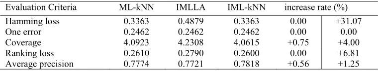
(3) Flags data set
Table 4. Contrast ML-kNN, IMLLA and improved IML-kNN (k=8). Evaluation Criteria ML-kNN IMLLA IML-kNN increase rate (%)
Hamming loss 0.3363 0.4879 0.3363 0.00 +31.07
One error 0.2462 0.2462 0.2462 0.00 0.00
Coverage 4.0923 4.2308 4.0615 +0.75 +4.00
Ranking loss 0.2610 0.2790 0.2600 0.00 +6.81
Average precision 0.7774 0.7721 0.7818 +0.56 +1.25
Indicator Figure and Analysis
The effect that three algorithms applied to three data sets respectively is shown in the figures below. We select three important indicators: Ranking Loss, Hamming Loss, Average precision as the vertical axis, three data sets as the horizontal axis, as shown in figure 1, figure 2, figure 3 respectively.
m
i y Y f i
i ' i f '
i f '
i i rank x,y
| Y ,y ,y x rank ,y
x |rank y | | |Y m f avgprec
1 ( )
} )
( )
( {
1 1 ) (
[image:4.612.116.497.558.630.2]Figure 1. Ranking Loss. Figure 2. Hamming Loss. Figure 3. Average precision.
It can be seen from the figures that improved IML-KNN algorithm is better than IMLLA algorithm, and is equal with or slightly better than ML-KNN algorithm on the Ranking Loss and Hamming Loss indicators, in terms of classification performance. IML-kNN improves a lot on the Average Precision index. In fact, the number of labels selected for each sample is small in the low potential data set, and the correlation between the labels is low, so the value of label set is much more depended on the k nearest neighbor sample than the correlation between labels. Therefore, we can improve the performance of ML-kNN classifier by considering the influence of the nearest neighbor sample.
Determining K Value and the Influence of K Value on the Improved Algorithm
How to determine k value: if k value is set too small, it will reduce the classification accuracy; if too large it will increase the noise. In this paper, the value interval of k is [8, 13], and then we use ten-fold cross-validation to determine a k value which show good classification performance in the training set.
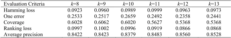
For each data set, we take k = 8, 9, ... , 12,13 respectively, and then use the improved IML-kNN algorithm to classify. Selecting the Scene data set to do the description, the other two data sets are similar.
Table 5. the influence of k value on the improved IML-kNN algorithm.
Evaluation Criteria k=8 k=9 k=10 k=11 k=12 k=13
Hamming loss 0.0923 0.0960 0.0989 0.0999 0.0963 0.0973
One error 0.2533 0.2517 0.2659 0.2492 0.2358 0.2441
Coverage 0.6028 0.6062 0.6020 0.5627 0.5368 0.5368
Ranking loss 0.0997 0.1002 0.0996 0.0919 0.0866 0.0868
Average precision 0.8422 0.8423 0.8379 0.8483 0.8560 0.8528
As can be seen from Table 5, multi-label classification is performed using formula (2) with nearest neighbor weights, where the effect of k on the classification results is the same as that of ML-kNN classification alone, i. e. for different data sets, a better value of the nearest neighbor k exists so that getting a better classification results in the five evaluation indicators.
Conclusion
In this paper, after making a deep study of the traditional ML-kNN algorithm, we propose a new and improved multi-label classification algorithm IML-kNN to solve problem that predicted accuracy using ML-kNN algorithm is not ideal for data set which has low coverage rate of labels selected. The advantage of improved algorithm is considering the influence of k neighbors and the nearest neighbor of unclassified sample simultaneously, and this effect is quantified by the weighted value. The simulation results show that the IML-kNN algorithm can achieve a better classification effect than ML-kNN and IML-kNN on some multi-label evaluation metrics.
Scene Medical Flags 0.05
0.1 0.15 0.2 0.25 0.3 0.35 0.4 0.45 0.5 0.55
Hamm
ing L
oss ML-KNNIMLLA IML-KNN
Scene Medical Flags
0.05 0.1 0.15 0.2 0.25
Ranking
Loss
ML-KNN IMLLA IML-KNN
Scene Medical Flags
0.72 0.74 0.76 0.78 0.8 0.82 0.84 0.86 0.88
Av
era
ge
Pre
cis
ion
ML-KNN IMLLA IML-KNN
[image:5.612.103.508.454.522.2]References
[1] Clare A., King R.D. knowledge discovery in multi-label phenotype data [M]//Principles of data mining and knowledge discovery. Springer Berlin Heidelberg, 2001: 42-53.
[2] Blockeel H., Schietgat L., Struyf J., et al. Decision trees for hierarchical multi-label classification: A case study in functional genomics [M]. Springer Berlin Heidelberg, 2006.
[3] Godbole S., Sarawagi S. Discriminative methods for multi-labeled classification[M]//Advances in knowledge Discovery and Data Mining. Springer Berlin Heidelberg, 2004: 22-30.
[4] Schapire R.E., Singer Y. BoosTexter: A boosting-based system for text categorization [J]. Machine learning, 2000, 39(2): 135-168.
[5] Jiang S., Pang G., Wu M., et al. An improved k-nearest-neighbor algorithm for text categorization [J]. Expert Systems with Applications, 2012, 39(1): 1503-1509.
[6] Markatopoulou F., Mezaris V., kompatsiaris I. A comparative study on the use of multi-label classification techniques for concept-based video indexing and annotation [C] // Multi-Media Modeling. Springer International Publishing, 2014: 1-12.
[7] Boutell M.R., Luo J., Shen X., et al. Learning multi-label scene classification [J]. Pattern recognition, 2004, 37(9): 1757-1771.
[8] Montañes E., Senge R., Barranquero J., et al. Dependent binary relevance models for multi-label classification [J]. Pattern Recognition, 2014, 47(3): 1494-1508.DOI: 10.1016.
[9] Hüllermeier E., Fürnkranz J., Cheng W., et al. Label ranking by learning pairwise preferences [J]. Artificial Intelligence, 2008, 172(16): 1897-1916.
[10] De Comité F., Gilleron R., Tommasi M. Learning multi-label alternating decision trees from texts and data [M]//Machine Learning and Data Mining in Pattern Recognition. Springer Berlin Heidelberg, 2003: 35-49.
[11] Elisseeff A., Weston J. A kernel method for multi-labeled classification [C] // Advances in neural information processing systems. 2001: 681-687.
[12] Zhang M.L., Zhou Z.H. ML-kNN: A lazy learning approach to multi-label learning [J]. Pattern recognition, 2007, 40(7): 2038-2048.
[13] Garcia E.K., Feldman S., Gupta M.R., et al. Completely lazy learning [J]. knowledge and Data Engineering, IEEE Transactions on, 2010, 22(9): 1274-1285.
[14] Minling Z. An Improved Multi-Label Lazy Learning Approach [J]. Journal of Computer Research and Development, 2012, 11: 002.
[15] Zhang M.L., Peña J.M., Robles V. Feature selection for multi-label naive Bayes classification [J]. Information Sciences, 2009, 179(19): 3218-3229.