Interferograms analysis for wavelength scanning interferometer using convolution and fourier transform

University of Huddersfield Repository

Muhamedsalih, Hussam, Jiang, Xiang and Gao, F.

Interferograms analysis for wavelength scanning interferometer using convolution and fourier 

transform.

Original Citation

Muhamedsalih, Hussam, Jiang, Xiang and Gao, F. (2009) Interferograms analysis for wavelength 

scanning interferometer using convolution and fourier transform. In: Proceedings of Computing and 

Engineering Annual Researchers' Conference 2009: CEARC’09. University of Huddersfield, 

Huddersfield, pp. 33­37. ISBN 9781862180857 

This version is available at http://eprints.hud.ac.uk/id/eprint/6858/

The University Repository is a digital collection of the research output of the

University, available on Open Access. Copyright and Moral Rights for the items

on this site are retained by the individual author and/or other copyright owners.

Users may access full items free of charge; copies of full text items generally

can be reproduced, displayed or performed and given to third parties in any

format or medium for personal research or study, educational or not­for­profit

purposes without prior permission or charge, provided:

•

The authors, title and full bibliographic details is credited in any copy;

•

A hyperlink and/or URL is included for the original metadata page; and

•

The content is not changed in any way.

For more information, including our policy and submission procedure, please

contact the Repository Team at: [email protected].

INTERFEROGRAMS ANALYSIS FOR WAVELENGTH SCANNING

INTERFEROMETER USING CONVOLUTION AND FOURIER-TRANSFORM

H. Muhamedsalih, X. Jiang And F.Gao

University of Huddersfield, Queensgate, Huddersfield HD1 3DH, UK

ABSTRACT

A convolution and fast Fourier transform methods are proposed separately to analysis a set of interferograms obtained from measurement results of a wavelength scanning interferometer. This paper describes wavelength scanning interferometer setup and the operation principle. Mathematical explanations,

for both interferograms analysis methods, are presented. Results of measuring 3μm step height sample,

using both interferograms analysis methods, are demonstrated. The results show that the convolution method provides better evaluation for the surface profile than the fast Fourier transform.

KeywordsConvolution; FFT; interferometry; interference fringes

1 WAVELENGTH SCANNING INTERFEROMETRY SYSTEM

The interferometry system, shown in figure 1, is composed of a Linnik interferometer illuminated by a halogen white light source, acousto-optic tuneable filtering and interface cards (i.e. DAQ and frame grabber) to communicate between the PC and the optical system. A 3μm step height calibrated sample is measured by the proposed system to verify the analysis methods. The Halogen white light is passed through an acousto-optic tuneable filter (AOTF). The function of AOTF is to act as a dynamic band pass filter to diffract instant selective wavelength into the interferometer and block the entire spectral band. The light wavelength that diffracts from AOTF was scanned from 680.8nm to 529.8nm with 0.5nm interval step. During the wavelength scanning process, 300 interferograms have been captured hence every interferogram has a specific wavelength. Every pixel in an interferogram represents a specific point upon the surface of a measured sample. So by isolating the pixels of a specific point on the sample; a sinusoidal intensity distribution can be obtained as shown in figure 2.a. Equation 1 describes the mathematical expression of the intensity distribution as stated by Hariharan in 2003.

(i)) cos( 2 I 1 I 2 ) i

λ

y; (x, 2 I ) i

λ

y; (x, 1 I

I(i)= + + ϕ …(1)

Where I1 and I2 are the intensities of measurement and reference beams respectively. The x and y refer to

the position of a pixel in the CCD. λi is the scanned wavelength and I is the iteration of the wavelength

scanning. φ is the phase of the intensity distribution that contains the required sample step height information. The phase of the intensity distribution depends on the wavelength and the optical path difference (i.e. height of the measured sample), as described in equation 2:

h * 2 i

λ

2π

(i)=

ϕ …(2)

λi is the scanning wavelength and h is the sample step height. Convolution and FFT algorithms have been

used to extract the point elevation from the intensity distribution.

2 CONVOLUTION ANALYSIS METHOD

The principle of convolution method is based on determining the positions of peaks or valleys obtained from intensity distribution, figure 2.a, with respect to the scanning wavelength. In this paper, the peaks have been considered. In order to calculate the step height (h) of the sample, the number and positions of peaks with respect to the scanning wavelength should be determined from the intensity distribution.

Applying convolution analysis to the intensity distribution is equivalent to calculate the first derivate of the distribution and low pass filtering of the high frequency noise contained in the distribution. The convolution process can be described through equation 3.

∫ −

= ₀2BI(x τ)f(τ)dτ

f(t) *

⎩ ⎨ ⎧ < < < < − = 2B t B 1 B t 0 1 f(t) …(4)

Where 2B is width of the function f(t) which is approximately equal to 74% of the mean intensity distribution wave period as described by Snyder in 1980.

Thus, by monitoring the change in the sign of the derived intensities data, the peaks positions can be determined when the intensity distribution is changed from negative to positive value.

Mathematically, the phase change between two successive peaks is 2π. So by subtracting phases at two specific peaks, the step height (h) can be obtained as the following:

) σ (σ * 4π 2π * 1) peaks of (number h 2 1 − −

= …(5)

Where σ1=1/λ1, σ2=1/λ2 and (λ1 & λ2)are the wavelengths at the selected peaks.

By applying equation 5 on every intensity distribution obtained from the interferograms, surface profile of the sample can be obtained. To optimize the sample surface profile measurement, the peaks positions (i.e. σj )

can be estimated more precisely by using linear interpolation method, and the step height (h) can be evaluated by using least-squares fitting approaches as proposed by Schwider et al in 2004. Equation 6 can be applied on the convoluted intensity distribution, as a linear interpolation fitting.

(r) 'I 1) (r 'I (r) 'I r ' r + + +

= …(6)

Where r’ _{is the actual position of a peak, I}’_{(r) is a negative sign magnitude of convolution output that followed}

by positive sign value, I’_{(r+1) is a positive sign magnitude of convolution output that led by negative sign}

value. Equation 7 can be used, as a least squares approach, instead of equation 5 to calculate the sample step height. ⎥ ⎥ ⎦ ⎤ ⎢ ⎢ ⎣ ⎡ ∑ = − + ∑+ − + = n 1 j n 1 j σj 1) (n j jσ 2 12 1) 1)(n n(n

h …(7)

Where j is the iteration of peaks or valleys (i.e. 0, 1, 2, 3,…,n),n is the number of peaks and σj=1/λj is the

wave number and λj are the wavelengths of the corresponding peak.

3 FOURIER TRANSFORM ANALYSIS METHOD

The same interferograms obtained from the interferometry have been analyzed using FFT. In contrast with convolution method, the slop of the intensity distribution attenuation needs to be compensated before FFT take place as stated by Takeda in 1982. The compensation has been achieved by dividing the intensities distribution of every pixel over the background intensity as shown in figure 2.b. The background intensity can be obtained by measuring the intensity variation of a pixel in the interferometer reference arm at the whole scanned wavelengths range.

The mathematical expression of equation1, can be rewritten in the following form for the convenience of explanation:

ϕ ϕ _Be i

2 1 i e B 2 1 A ) i

I(λ = + − − …(8)

WhereA=I1(x,y;λ)+I2(x,y;λ) and B=2 I₁(x,y;λ)I₂(x,y;λ)

To simplify the above equation, the following notations can be considered:

ϕ

i e 2 1

c= and e iϕ 2 1 *

c =− −

FFT can be applied to equation 9 to find the spectrum of the intensity distribution. The purpose of FFT is to distinguish between the useful information which is represented by the phase change (i.e. c or c* term) and the unwanted information which is represented by the DC bias (i.e. A).

) i λ B(f, c ) i λ B(f, c ) i λ A(f, )] i [I(λ

FFT = + + ∗ …(10)

The unwanted amplitude variation A and c∗ has been filtered out and the inverse FFT was applied to the filtered signal cB(f,λi). So the FFT outcome is B½ eiφ.

Furthermore, complex logarithm has been applied to B½ eiφ in order to separate the phase φ from the unwanted amplitude variation B, as illustrated in equation 11.

ϕ

ϕ _{B] i}

2 1 [ ln ] i e 2 1

ln[B = + …(11)

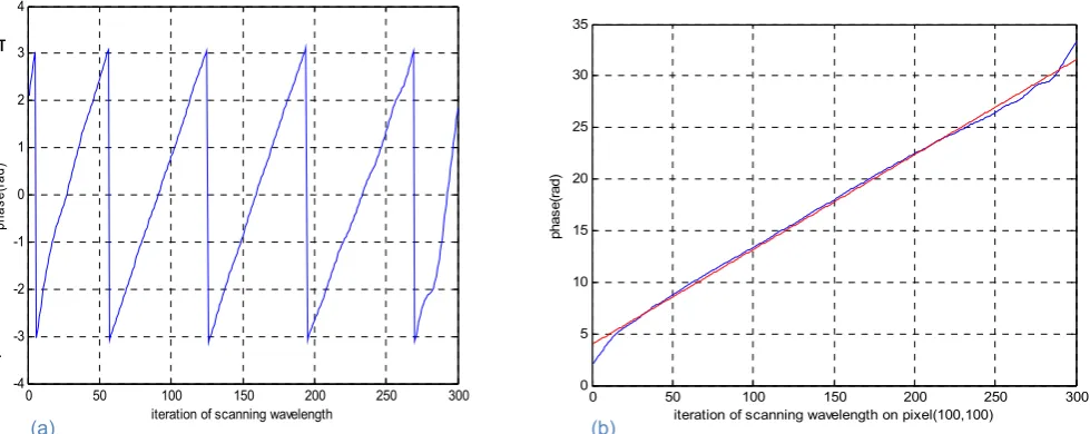
The phase was extracted from the imaginary part of equation 11, and Figure 3.a has been obtained. Figure 3.a suffers from discontinuities, where the values are in the range from –π to π. These discontinuities have been corrected by adding 2π at the discontinuous points to obtain continuous phase distribution as shown in figure 3.b. Finally, by using the continuous phase distribution and equation 12, the sample step height can be calculated.

⎥ ⎥ ⎦ ⎤ ⎢

⎢ ⎣ ⎡

− =

n λ

1 m λ

1 4π

∆

h ϕ …(12)

Where ∆φ is the change in phase between any two points in figure 3.b. λm and λn are the corresponding

wavelengths phase difference (∆φ). 4 RESULTS AND DISCUSSION

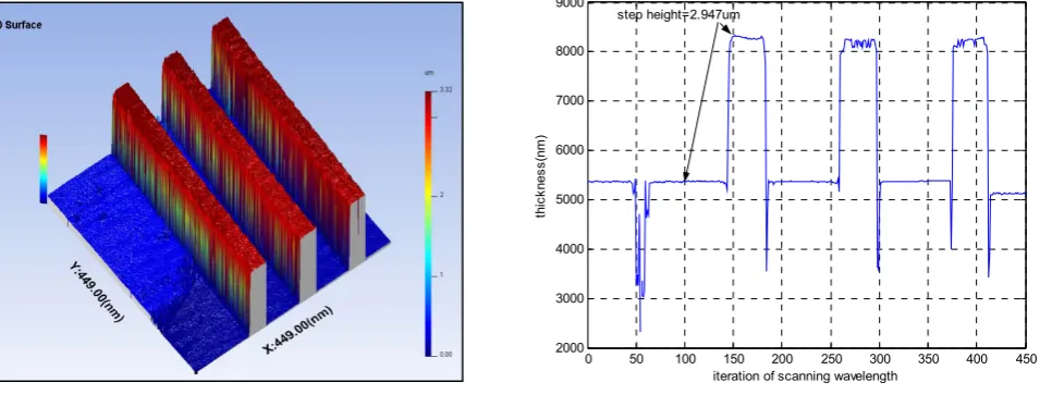
The convolution analysis method was applied to the interferograms obtained from the interferometry described in section1. The measurement of the sample step height, using equation 5, was 2.979μm. This measurement was improved when the linear interpolation and least squares fitting methods were introduced to convolution analysis. The measurement error has been reduced from 0.7% to 0.43% where the step height measurement was 2.987μm as shown in figure 4.

The same interferograms have been processed using FFT. It was found that the calculated phase calculation has discontinuity when the variation exceeds 2π value as shown in figure 3.a. The discontinuous data has been corrected as shown in figure 3.b. The measurement of the sample step height was 2.947μm as shown in figure 5. It was found that the main reason that causes an error for the measurement, using FFT analysis, is the variation and attenuation in the light intensity when the light wavelength is shifted to shorter wavelength band.

5 CONCLUSION

An optical system for wavelength scanning interferometry has been introduced to measure discontinues surface profiles without phase ambiguity. The principle of the interferometry based on using a white light spectral scanning interferometry together with acousto-optic tuneable filtering.

A convolution and Fourier transform methods have been proposed and verified by analyzing the interferograms obtained from interferometry. The convolution results show better accuracy than using Fourier transform to evaluate the surface profile. The average measurement error of convolution is 0.7%. The convolution error has been reduced to 0.43% by using linear interpolation and least squares fitting methods. While the average measurement error using Fourier transform is 1.7%. The Fourier transform measurement has been obtained after removing the irradiance variation and compensating for the phase discontinuities.

REFERENCES

HARIHARAN P. (2003), Optical Interferometry, Elsevier-USA, 2nd edition, p.11.

SCHWIDER J., ZHOU L. (1994), Dispersive Interferometric Profilometer, Optics Letters, Vol.19, No.13, pp.995-997.

TAKEDA M., INA H. and KOBAYASHI S. (1982), Fourier-Transform Method of Fringe Pattern Analysis for

Computer based Topography and Interferometry, Optical Society of America, Vol.72, No.1, pp.156-160.

[image:5.595.156.401.94.259.2]

Figure 1 basic configuration of the proposed surface measurement system

0 50 100 150 200 250 300

50 100 150 200

0 50 100 150 200 250 300

130 140 150 160 170 180 190 200 210

iteration of scanning wavelength for pixel (100,100) iteration of wavelength scanning

light

in

tens

ity

(

lm

) )

ity

(l

m

t i

nt

ens

ghli

Figure 2 (a) intensity’s distribution for pixel (100,100) for 300 interfergrams (b) corrected intensity distribution for the same pixel

0 50 100 150 200 250 300

0 5 10 15 20 25 30 35

iteration of scanning wavelength on pixel(100,100)

pha

se

(r

ad)

π

-π

0 50 100 150 200 250 300

-4 -3 -2 -1 0 1 2 3 4

phas

e(

ra

d)

iteration of scanning wavelength

(a) (b)

[image:5.595.46.528.318.500.2] [image:5.595.43.533.565.760.2]

0 50 100 150 200 250 300 350 400 450 1000

2000 3000 4000 5000 6000 7000 8000 9000 10000

T

hi

ckn

ess (

nm

)

Step height=2.987um

pixels' iteration in x dimension whereas py=100 Step height measurement using convolution method

a) (b)

Figure 4 (a) 3D step height measurement of the 3μm standard sample using convolution method. (b) 2D surface profile measurement

0 50 100 150 200 250 300 350 400 450

2000 3000 4000 5000 6000 7000 8000 9000

iteration of scanning wavelength

th

ickn

ess(

nm

)

step height=2.947um

(a)

[image:6.595.58.527.74.267.2] [image:6.595.51.529.300.487.2]