Geometric computation theory for morphological filtering on freeform surfaces

Geometric computation theory for morphological filtering

on freeform surfaces

By Shan Lou, Xiangqian Jiang*, Paul J. Scott

EPSRC Centre for Innovative Manufacturing in Advanced Metrology, University of Huddersfield, Queensgate, Huddersfield, HD1 3DH, UK

*Corresponding author: Tel: +44 1484 473634; Fax: +44 1484 472161; E-mail:

x.jiang@hud.ac.uk

Surfaces govern functional behaviours of geometrical products, especially high precision and high added-value products. Compared to the mean-line based filters, morphological filters, evolved from the traditional E-system, are relevant to functional performance of surfaces. The conventional implementation of morphological filters based on image processing does not work for state-of-the-art surfaces, for example freeform surfaces. A set of novel geometric computation theory is developed by applying the alpha shape to the computation. Divide and conquer optimisation is employed to speed up the computational performance of the alpha shape method and reduce memory usage. To release the dependence of the alpha shape method on the Delaunay triangulation, a set of definitions and propositions for the search of contact points is presented and mathematically proved based on alpha shape theory, which are applicable to both circular and horizontal flat structuring elements. The developed methods are verified through experimentation.

Keywords: morphological filters, surface analysis, contact points, computational geometry, alpha shape.

1. Introduction

The surface of a geometrical component is an interface limiting the body of the component and separating it from the surrounding medium. It governs the functional behaviours of the product, whether that be a mechanical, tribological, hydrodynamic, optical, thermal, chemical or biological property, all of which are of tremendous importance to product performance (Bruzzone et al. 2008; Jiang 2009;). Many emerging products and devices are based on achieving surfaces with special functionalities. Manufactured items such as micro- and nanometre scale transistors, micro electro mechanical systems (MEMS) and nano electro mechanical systems (NEMS), microfluidic devices, optics components with freeform geometry and structured surface products are clear evidence of products where the surface plays the functional role (Jiang et al. 2007).

Surfaces and their measurement, provide a link between the manufacture of these engineering components and their use (Whitehouse 1978). On the one hand, it can help control the manufacture process: monitor changes in the surface texture and indicate changes in the manufacturing process such as machine tool vibration and tool wear (Peters et al. 1979; Trumpold 2001). On the other hand, it can help with functional prediction: characterize geometrical features that will directly impact on tribology and physical properties of the whole system (Unsworth 1995; Sayles 2001; Whitehouse 2001), for instance, the friction of two contact surfaces and the optical fatigue of one reflecting surface.

called the roughness and the latter the waviness. Also, in addition to roughness and waviness, even longer wavelength can be introduced into the surface geometry by weight deflection or long-term thermal effects (Whitehouse 2002). Filtration techniques are the means by which roughness, waviness and form components of the surface texture are extracted from the measured data for further characterization. By separating surface profile into various bands, it is possible to map the frequency spectrum of each band to the manufacturing process that generated it (Raja et al. 2002). Filtration techniques are also widely used in dimensional metrology to suppress the noises in the measured data to achieve a more stable data set.

The 1950s saw two attempts to separate the waviness from the profile so that the roughness could be characterised. One was graphical, simulating electrical filters in the meter circuit (Whitehouse & Reason 1965). The raw profile was divided into segments of equal length, and in each segment a mean line was drawn that captures the slope of the profile in that segment. The roughness profile was obtained by considering the deviation from the mean line. Thus it was designated the mean line system (M-system). The other was mechanically simulating the contact of a converse surface, e.g. a shaft, with the face of the anvil of a micrometer gauge (Von Weingraber 1956). It appeared as a large circle rolling across over the profile from above and was entitled the envelope system (E-system).

The E-system based the reference line upon an envelope generated by the centre of a rolling circle and shifted to the average height of the profile (Thomas 1999). The difficulty appeared in building practical instruments as two elements are needed: a spherical skid to approximate the “enveloping circle” and a needle-shaped stylus moving in a diametral hole of the skid to measure the roughness as deviation with respect to the “generated envelope”. The advantage of the E-system was claimed to be that it is more physically significant in that many engineering properties of a surface are determined by its peaks (Peklenik 1973). However, the standing objection was that the choice of the rolling circle radius is as arbitrary as the choice of cut-off in the M-system and no practical instruments using mechanical filtering could be made at that time. The discussion about the reference systems lasted for at least one decade between 1955 and 1966 (Peters 2001). Around 1960, with the advent of digital processing techniques, the M-system became pre-eminent and was improved by the 2RC digital filter and phase-corrected digital filter. Later the Gaussian filter, with better performance, was chosen as the standardized filter for separating differing wavelengths.

The Gaussian filter, although a good general filter, is not applicable for all functional aspects of a surface, for example in contact phenomena, where the E-system method is more relevant. The advent of fast practical computers, which can be used in association with measurement instruments, had virtually eliminated the need for any hardware implementation for the E-system (Tholath & Radhakrishnan 1999). Furthermore, there were growing evidences showing that the E-system method can give better results in functional prediction of surface finish in the analysis of mating surfaces, such as contact, friction, wear, lubrication and failure mechanism (Westberg 1997). With the M-system, there is little correlation between the standardized surface roughness parameters and functional requirements, while the E-system that depends on geometrical characteristics of the workpiece is more relevant (Dietzsch et al. 2008). In this aspect the logic of the E-system was sounder as against the M-system. Both the M-system and the E-system approaches have their benefits and limitations. Arguing that one is better than the other without any concrete proof from the application area is not convincing (Radhakrishnan & Weckenmann 1998). In fact rather than competing with each other, the M-system and the E-system are complementary to each other, contributing to a better solution to surface evaluation.

regression filter (Seewig 2006; Zeng et al. 2010), the spline filter (Krystek 1996), and the robust spline filter (Goto et al. 2005; Zeng et al. 2011). More recently, a method of Gaussian filtering for freeform surface was developed by solving the diffusion equation which overcomes geometrical distortion in the presence of non-zero Gaussian curvature (Jiang et al. 2011).

Meanwhile the E-system also experienced significant improvements. By introducing mathematical morphology, morphological filters emerged the superset of the early envelope filter, but offering more tools and capabilities (Srinivasan 1998). The basic variation of morphological filters includes the closing filter and the opening filter. They could be combined to achieve superimposed effects, referred to as alternating symmetrical filters. Scale-space techniques further developed morphological filtering techniques, which provide a multi-scale analysis to surface textures (Scott 2000). Even though morphological filters are generally accepted and regarded as the complement to mean-line based filters, they are not universally adopted due to limitations caused by their current implementation and lack of capabilities demanded by the analysis of modern functional surfaces, especially freeform surfaces.

Freeform surfaces are continuous surfaces having no translational and rotational symmetry (ISO 17450-1 2011; Jiang & Whitehouse 2012). For freeform surfaces, the description data might be specified by coordinates in two or three dimensions, rather than regular surface height. Responding to all these requirements, novel methods based on the geometric computation have been developed with an aim of supporting morphological filtering on freeform surfaces. Alpha shape theory provides the theoretical basis of geometrically computing morphological envelopes. Furthermore the contact points on component surfaces are highly addressed for they play a critical role in determining morphological envelopes. The paper mainly exhibits the geometric computation theory for morphological filtering on freeform surfaces. Applications are also added to further illustrate the capability and feasibility of the proposed computation theory.

2. Morphological operations and morphological filters

2.1 Morphology operations on sets

Mathematical morphology is a mathematical discipline established by two French researchers Jorge Matheron and Jean Serra in the 1960s. An overview of their work is given in Serra (1982). The central idea of mathematical morphology is to examine the geometrical structure of an image by probing it with the structuring element. Four basic morphological operations, namely dilation, erosion, opening and closing, form the foundation of mathematical morphology.

Dilation combines two sets using the vector addition of set elements. The dilation of

A

by

B

is defined as:

D A B( , ) A B ∨

= ⊕ , (2.1)

where ⊕ is the vector addition and B ∨

is the reflection of B through the origin of B.

Erosion is the morphological dual to dilation. It combines two sets using the vector subtraction of set elements. The erosion of

A

by

B

is

( , )

E A B A B ∨

= , (2.2)

Both opening and closing use combinations of dilation and erosion operations in pairs. The opening of

A

by

B

is obtained by applying the erosion followed by the dilation with the common set element B,

( , ) ( ( , ), )

O A B D E A B B ∨

= . (2.4)

Closing is the morphological dual to opening. The closing of

A

by

B

is given by applying the dilation followed by the erosion,

( , ) ( ( , ), )

C A B E D A B B ∨

= . (2.5)

2.2 Morphological filters for surface metrology

Morphological filters in surface metrology are based on mathematical morphology. The profile and surface are treated as functions on and respectively (Srinivasan 1998). They are carried out by performing morphological operations on the input profile/surface with circular or horizontal flat structuring elements (ISO 16610-40 2010).

As Figure 1 illustrates, the dilation of the surface profile with a disk structuring element is the locus of the centre of the disk as it rolls over the profile from the above (Scott 2000). Dual to the dilation, the erosion is obtained by rolling the disk over the profile from the below. See Figure 2. Closing is the combination of two operations, first a dilation followed by an erosion. Opening is morphological dual to closing, given by applying an erosion followed by a dilation. In fact, the closing and opening envelope are the upper and lower boundary of the disks respectively. In particular, the E-system is a dilation envelope with a circular structuring element offset by the disk/ball radius.

It is obviously revealed that the closing filter suppresses the valleys on the profile which are smaller than the disk radius in size, meanwhile the peaks remain unchanged. On the contrary the opening filter suppresses the peaks on the profile which are smaller than the disk radius in size, while it retains the valleys. The combining effects of the closing and opening filter lead to alternating symmetrical filters, by which peaks and valleys are both suppressed.

2.3 Conventional computation method and limitations

This supporting algorithm, although easy in implementation, has a couple of limitations which restrict the prevalence of morphological filters. They are restricted to “planar surfaces”, namely height fields embedded in the Euclidean spaces and therefore unsuitable for freeform surfaces. Even with planar surfaces data, it is not robust against rotation in space. Another shortcoming lies in the destructive end effects for surfaces in the presence of significant form component, which is notable when the structuring element of a large size is used. As a result, the filtration will be badly distorted in the boundary regions.

[image:5.595.183.427.88.196.2]

A further issue regarding existing methods is their inaccuracy in capturing the contact points of the measured surface with the structuring element. The detection of contact points is dependent on the numerical comparison between the original data and the closing or opening

[image:5.595.173.431.253.367.2]

Figure 1. The dilation and closing envelope of an open profile by a disk.

Figure 2. The erosion and opening envelope of an open profile by a disk.

[image:5.595.188.401.593.747.2]

envelope. This is limited by the accuracy of the algorithm and sensitivity to the round-off errors in the calculation. This situation is even compounded by sampling the structuring element discretely.

Besides the limitations mentioned above, morphological filters also suffer from two practical issues raised in the employment of the traditional computation method. For areal surface datasets with large number of measured points, the method is extremely time-consuming. Even using the current available commercial surface analysis software, e.g. the Mountain map (Digital Surf), the performance is far from satisfactory. Also the size of the structuring element is restricted from growing big due to the fact that the computational time is in exponential proportion to the size of structuring element. For another, the image processing based methods treat the data as uniformly distributed pixels and unsuited to non-uniform sampled data. This further limits their usage in the field of dimensional metrology where adaptive sampling is allowed.

Except for the image processing based approach, there are a few other computation methods, which yet cannot fully overcome the aforementioned deficiencies (Scott 1992; Tholath & Radhakrishnan 1999; Kumar & Shunmugam 2006). In particular, Scott (1992) developed an efficient algorithm for morphological profile filters on the basis of motif combination. However it is hard to extend this idea to areal data.

3. The alpha shape method for morphological filters

To overcome the limitations of the traditional computation method, a totally different method has been developed, whereas measured surfaces are no longer treated as greyscale images, but 3D point clouds (Jiang et al. 2012). Geometric computation techniques are adopted to solve the morphological envelope of the point cloud. The alpha shape, a ubiquitous geometric structure in the field of surface reconstruction, is closely related to morphological envelopes and can be employed for their computation.

3.1 Alpha shape theory

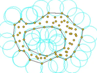
The alpha shape was introduced by Edelsbrunner in the 1980s aiming to describe the specific “shape” of a finite point set with a real parameter controlling the desired level of details (Edelsbrunner & Muche 1994). Given a planar point set, a circular disk of radius

α

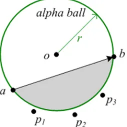
is rolled around both inside and outside (see Figure 4), this will generate an object with arcs and points. The boundary of the resulted object is called the alpha hull. If the round faces of the object are straightened by line segments, it generates another geometrical structure, the alpha shape. [image:6.595.237.394.624.743.2]

In the context of the alpha shape, the disk used in the above example is called the alpha ball. It is formally defined as an open ball of radius

α

. Given a point set X ⊆ , a certain

alpha ball b is empty if b∩X = ∅_{. With this, a k-simplex}

T

σ

is said to be α_{-exposed if}

there exists an empty alpha ball bwith T = ∂b∩X (T = +k 1) where ∂b is the surface of the sphere (for d=3) or the circle (for d=2) bounding b, respectively.

Definition 1. For 0≤

α

≤ ∞, the alpha hull of X , denoted by H_α( )X , is defined as the complement of the union of all empty α_{-balls. S (X)}

α

∂ , the boundary of the alpha shape of the point set X , consists of all k-simplices of X for 0≤ <k d which are α_-exposed,

( ) { | , 1, α_-exposed}

T T

S_α X

σ

T X T k

σ

∂ = ⊂ = + (3.1)

The computation of the alpha shape is based on the Delaunay triangulation. Given a point set X ⊆ , the Delaunay triangulation is a triangulation DT X( ) such that no point in X is inside the circumsphere of any d-simplices

T

σ

with T ⊂ X . The relationship between the Delaunay triangulation and the alpha shape is that the boundary of the alpha shape ∂S_α is a subset of the Delaunay triangulation of X , i.e.

( ) ( )

S_α X DT X

∂ ⊂ . (3.2)

In order to further extract the simplices of ∂S_α(X) from DT X( ), another concept, the alpha complex C_α(X), was developed. Set

ρ

_T the radius of the smallest circumsphere b_T of

T

σ

. For k=3, b_T is the circumsphere; For k=2, b_T is the great circle; And for k =1, the two points in

T

are antipodal on b_{T. For a given point set} X ⊆ , the alpha complex

( )

C_α X is the following simplicial sub-complex of DT X( ).

A simplex

σ

_T∈DT X( ) (

T

= +

k

1

, 0≤ ≤k d) is in C_α(X) if:

(1)

ρ

_T <

α

and

ρ

_T-ball is empty, or

(2)

σ

_T is a face of other simplex in C_α(X).

The relationship between the alpha complex and the alpha shape is that the boundary of the alpha complex makes up the boundary of the alpha shape, i.e.

( ) ( ) ( )

C_α X S_α X DT X

∂ = ∂ ⊂ . (3.3)

3.2 Link between alpha hull and morphological envelopes

The alpha hull resembles the morphological opening and closing envelopes, as the alpha ball acts as a spherical structuring element and the input set as the point set. In fact a theoretical link between the alpha hull and morphological opening and closing operations was found by Worring and Smedulers (1994) that the alpha hull is equivalent to the closing of X with a generalized ball of radius −1

α

. Hence from the duality of the closing and the opening, the alpha hull is the complement of the opening of Xc (complementation of X ) with the same ball as the structuring element.

3.3 Morphological envelope computation based on the alpha shape

The Delaunay triangulation results in a series of k-simplices

σ

(k =2 for profiles, which are triangles; k =3 for surfaces, which are tetrahedrons). These k -simplices are categorized into two groups: k-simplices

σ

p whose circumsphere radius is larger than the

radius of the rolling ball

α

, and k-simplices

σ

_np whose circumsphere radius is no larger than the radius of the rolling ball

α

.

p

σ

consists of two parts: the

(

k

−

1)

-simplices

σ

_int interior to

σ

_p, and the

(

k

−

1)

-simplices

σ

_reg that bounds its super k-simplices

σ

_p. We called

σ

_reg the regular facets.

σ

_np is comprised of three components: the

(

k

−

1)

-simplices

σ

_ext out to C_α, part of the regular facets

σ

_reg' shared by both

σ

pand

σ

np, and the

(

k

−

1)

-simplices

σ

sing that are the other

part of ∂C_α. We call

σ

_sing the singular facets.

σ

_sing differs from

σ

_reg in that it does not bound any super k-simplices belonging to C_α.

σ

_sing satisfies two conditions as follows:

(1) The radius of its smallest circumsphere is smaller than

α

. (2) The smallest circumsphere is empty.

An explanatory graph is presented by Figure 5. The regular facets

σ

_reg and the singular facets

σ

sing form the whole boundary of the alpha complex, i.e. the boundary of the alpha

shape, as the equation (3.4) presents.

reg sing

S

_α

C

_α

σ

σ

∂

= ∂

=

+

(3.4)

Figure 6 illustrates an example of the alpha shape facets extracted from the Delaunay triangulation of an experimental profile data. With the boundary alpha shape facets, the morphological envelope can be solved. For each sample point, there is a one-to-one corresponding point on the envelope. These points form a discrete representation of the morphological envelope. Each boundary facet of the alpha shape determines its counterpart on the alpha hull. Due to the fact that the target envelope is contained in the alpha hull, the sample points are projected onto the alpha hull along the local gradient vector to obtain the envelope coordinates.

[image:8.595.160.449.613.756.2]

The alpha shape method calculates morphological filters geometrically and has a number of advantages over traditional methods. Firstly, by viewing the measured surface points as the 2D/3D point set, it breaks the constraints of the traditional method which only applies to planar profiles/surfaces. Secondly, alpha shape theory enables arbitrary size of disk/ball radius. Moreover, the alpha shape method more suits non-uniform sampled data. The alpha shape method depends on the Delaunay triangulation, bringing in an additional merit that the

triangulation could be reused for multiple attempts of various disk radii, saving a great deal of computing time because in practice a multitude of trials may be made for choosing an appropriate disk radius.

3.4 Divide and conquer optimisation

The alpha shape method is more competent than traditional algorithms. However its bottleneck is that the 3D Delaunay triangulation is costly in both computation time and memory for large areal data sets and it was reported that the data structure of the Delaunay triangulation is not suitable for datasets of millions of points (Bernardini et al. 1999). In practice, measured engineering surfaces usually contain a large quantity of data, especially using fast optical measurement instruments. As a result, the divide and conquer optimisation is employed to speed up the computation of morphological envelopes and avoid the risk of running out of memory.

In the context of the alpha shape method, the vertices of boundary facets of the alpha shape are of tremendous importance because they are the surface points in contact with the rolling ball. The morphological envelope of a surface is only determined by these vertices, while not affected by other points.

The basic scheme of the divide and conquer approach is to break a problem into several problems that are similar to the original problem but smaller in size, solve the sub-problems iteratively and then combine these solutions to create a solution to the original problem (Cormen et al. 1989). By applying the divide and conquer method, the surface under evaluation is divided into a series of small sub-surfaces. Each sub-surface is rolled by the ball to generate a set of alpha shape vertices. Afterward the resulted vertices from each sub-surface are merged to reconstruct a super set of vertices, which will be treated as the point set for the next iteration. It will be noticed that some of the vertices around the joint sections in the previous iteration are removed. By repeating the iterations, the final alpha shape of the original surface can be found and the morphological envelope of the surface is then determined. A demonstration of the divide and conquer procedures is given by Figure 7.

4. The contact points and their searching procedures

Using the alpha shape vertices, the divide and conquer optimisation reduces the amount of points in the iteration processed by the Delaunay triangulation. However it is not a fundamental change to the alpha shape method because the Delaunay triangulation is still required in order to extract the alpha shape boundary facets. It will be revealed that the Delaunay triangulation is not necessary for searching the boundary facets and an alternative computational method is explored by searching the contact points.

4.1 Redundancy of the Delaunay triangulation

[image:10.595.136.463.81.492.2]

In Edelsbrunner’s theory the alpha shape is extracted from the Delaunay triangulation. In fact the whole family of alpha shapes can be generated from the Delaunay triangulation, from the point set itself (

α

→0) to the convex hull of the point set (

α

→ ∞). Therefore the Delaunay triangulation data could be reused for multiple attempts of ball radii for the same data set. It however could be a drawback because the Delaunay triangulation is costly for large areal data sets. Given a single radius, the Delaunay triangulation contains much more information than

is necessary to generate the corresponding alpha shape for that radius. Thus in this sense it is a waste of time and memory to achieve the desired alpha shape with redundant computation.

4.2 Definition of contact points

In physics, the contact points are those points on the surface which are in contact with the moving structuring element. Thus these points give an indication which surface portions in the neighbourhood of these contact points are most likely to be active in the contact phenomenon. From a point of view of mathematical morphology, the contact points are those points on the surface which remain constant before and after morphological closing/opening operations. Based on the mapping between the alpha hull and morphological opening and closing envelopes, the formal mathematical definition of the contact point is given by Definition 2 using alpha shape theory:

Definition 2. Given a sampled point setX ⊆

(

d

=

2, 3)

and

δ

≤

α

≤ ∞(

δ

: sampling

interval), the contact points

P

( )

α

are those sampled points {p_i|p_i∈X} that are on the boundary of the alpha hull ∂H_α(X):

{

}

( ) _i | _i , _i ( )

P

α

= p p ∈X p ∈ ∂H_α X .

4.3 Propositions for searching contact points

Proposition 1. Given a point set X ⊆

(

d

=

2, 3)

and

δ

≤

α

₁≤ ∞ ,

δ

≤

α

₂ ≤ ∞ , if

1 2

α

≤

α

, then P(

α

₂)⊆P(

α

₁). Proof.

1 2 1 2

H

α

( )

X

H

α

( )

X

α

≤

α

⇒

⊆

_{(Fischer 2000). By Definition 2,}

{

1

}

1

(

)

_i

|

_i

,

_i

( )

P

α

=

p

p

∈

X p

∈ ∂

H

_α

X

,

{

}

2 2

(

)

_i

|

_i

,

_i

( )

P

α

=

p

p

∈

X p

∈ ∂

H

_α

X

. Hence

1

( )

2

( )

H

_α

X

⊆

H

_α

X

implies P(

α

₂)⊆P(

α

₁).

Proposition 2. Given the point set X ⊆

(

d

=

2, 3)

and

δ

≤

α

≤ ∞. The convex hull points must all be contact points.

Proof. Let

α

′ → ∞ , hence lim_α′→∞H_α′(X)=Conv X( ) . By Definition 2,

{

}

( ) _i| _i , _i ( )

P

α

′ = p p ∈X p ∈ ∂H_α′ X , then P(

α

′ =)

{

pi|pi∈X p, i∈ ∂Conv X( )

}

, namely

(

)

P

α

′

is the convex point set. By Proposition 1,

α α

≤

′

⇒

P

( )

α

′

⊆

P

( )

α

_{. Thus the convex}

hull points must be contained in

P

( )

α

.

Figure 8 presents an example illustrating the boundary facets of the alpha shape of a planar point set regarding to four different disk radii respectively. The Delaunay triangulation of the point set is presented by triangle mesh and the boundary facets of alpha shape are graphed as bold dotted lines. It can be easily verified that the results presented by four sub-figures are consistent with Proposition 1 and 2. For instance, the contact points of Figure 8(a) with radius 1 mm are contained in Figure 8(b) with radius 0.5 mm, and so forth.

Proposition 3. If there are points lying above

σ

_ab (left/positive side of ab), then the contact point is the furthest point orthogonal to ab. [image:12.595.122.471.78.362.2]

Proof. Suppose there exist some points above

σ

_ab. See Figure 9. The furthest point c is the convex point for the point set { , , ,a b c p_i} (Barber et al. 1996). By Proposition 2, the convex point must be the contact point. Thus c must be the contact point.

Figure 9. Search the furthest point on the positive side of ab in orthogonal direction.

Proposition 4. If there are no points lying above

σ

_ab and there exist points { }p_i in the circular section of the ball with radius 1

2

max{ ,r ab}

[image:12.595.197.397.547.679.2]

α

= , then the contact point c is the Figure 8. The Delaunay triangulation of a planar point set and the boundary facets of the alpha shapes of four disk radii: (a) mm; (b) mm; (c) mm; (d)

one among the points { }p_i in , which satisfies the condition: the circumscribed circle of

abc

σ

have the largest radius among the circumscribed circles of

{

}

i

abp

σ

.

Proof. First consider the case ab ≤2r. See Figure 10(a). a, b could determine an unique alpha ball B with radius

r

. Since there exist points in the circular section (the shadowed portion in the figure), B∩X ={ }p_i ≠ ∅ , thus

σ

_ab is not α_{-expose. By Definition 1,}

( ) ab H Xr

σ

∉ ∂ . Let { }

ρ

_i be the radii of the circumscribed circles of

{

}

i

abp

σ

and c the point with max(

ρ

_i) . The circumcircle of

σ

_abc must be empty, thus _{max( )}

( )

i

c

∈ ∂

H

_ρ

X

. By

Proposition 1, max(

ρ

_i)>r⇒P(max(

ρ

_i))_⊆P r( )_{. By Definition 1, (max( ))} i

c∈P

ρ

. Thus

c

∈

P r

( )

, c is the contact point.

Then consider the other case ab >2r. See Figure 10(b). Since ab >2r, fit a great

circle with radius 1 2 ab

α

= passing through the points a, bwith the centre at the middle of

ab

σ

. Similar to the previous case, we could prove 1 2

( )

c∈P ab . Then by Proposition 2,

1 1

[image:13.595.112.482.338.538.2]

2 ab >r⇒P( 2 ab)⊆P r( ), thus

c

∈

P r

( )

, c is the contact point.

Figure 10. Search the contact point with: (a) ab ≤2r; (b) ab >2r.

Definition 3.

{ }

p_i are points lying below

σ

_ab (right/negative side of ab).

i

abp

σ

has an unique circumscribed circle with radius

α

. If the centre of the circumscribed circle is on the positive side of

σ

_ab, the circle has the positive radius +

α

, otherwise the negative radius −

α

.

See Figure 11.

{

p p p₁, , ₂

}

are three points below

σ

_ab. 1

abp

σ

has its circumcircle centre

1

o above

σ

_ab, thus it has a positive radius. Conversely, the centre of the circumcircle of

2

abp

[image:14.595.205.385.69.248.2]

Figure 11. The signed circumscribed circle radius.

Proposition 5. If ab >2r and there are no points lying above

σ

_ab and also no points in the circular section of the alpha ball with radius 1

2 ab

α

= , then the contact point is the one

c that satisfies the condition: the circumscribed circle of

σ

_abc has the largest radius among the circumscribed circles of

{

}

i

abp

σ

.

Proof. See Figure 12. There is no point in the circular section , thus the centre of

circumscribed circles of

{

}

i

abp

σ

locates at the negative side of the chord ab. Thus their radii are negative. The circumscribed circle with the largest radius (smallest in absolute value) must be empty, thus c∈ ∂H_α( )S .

α

>r⇒c∈ ∂H S_r( ) _{. By Proposition 1, we have}

( )

c

∈

P r

.

Figure 12. Search the contact point with ab >2r and empty.

Proposition 6. If ab ≤2r and there are no points lying above

σ

_aband also no points in the circular section of the alpha ball with radius

r

, then

σ

_ab∈ ∂H X_r( ).

Proof. See Figure 13. a, b could determine an alpha ball B with radius r. If there is no point lying above

σ

_ab and no point in the circular section , then ∂B∩X =

{

a b,

}

. Thus

ab

σ

is α_{-expose. By Definition 1, ( )}

ab H Xr

[image:14.595.232.364.455.606.2]

[image:15.595.235.362.75.202.2]

Figure 13.

σ

_ab determines a facet of the alpha shape.

Propositions 1-6 establish the searching order of contact points. It first targets convex hull points between two known contact points, which corresponds to rolling a disk with an infinite large radius over the profile. If no convex hull point lies above the evaluating simplex, the contact point is found by computing the signed circumcircle radii. The contact point is the one that has the largest circumcircle radius. This is equivalent to rolling a disk with a radius smaller than the infinite big but larger than the given radius

r

. Finally if the simplex in evaluation could hold an empty disk with radius

r

by its two ends, namely the disk is in no contact with other sample points except two end points, then the simplex is a boundary facet of the alpha shape. In summary the algorithm is searching the contact points using disks with radius ranging from the infinite big down to

r

. It should be notified that the above propositions also hold for areal data by replacing the disk with a ball and the circumcircle with a circumsphere.

Although the presented algorithm is specific to circular structuring elements, it is even easier to apply the basic scheme to horizontal flat structuring elements. In that case, the contact point is examined by checking the highest point (say p₂ in

{

p p p₁, ₂, ₃

}

) between two known contact points (say a, b). If that point is lower in height than two given contact points (say p2 is lower than a, b) and the horizontal distance between the two contact

points is smaller than the length of the given horizontal line segment (say ab <L), the

searching procedure exits and the envelope height is determined by the lower height of the two contact points.

5. Performance comparison

Using the traditional method, the calculation of each envelope coordinate will involve the whole surface data when the size of structuring element is equal and larger than that of the surface, thus its time complexity is O n( 2). The alpha shape depends on the Delaunay triangulation, which has the theoretical time complexity of

O n

( log )

n

. The divide and conquer optimisation, although still relying on the Delaunay triangulation, can reduce the amount of points being processed in the iteration and require less computation memory. The contact point searching method eliminates the dependence of the alpha shape method on the Delaunay triangulation, having the expected time complexity

O n

( log )

n

.

12 hours for the 1000

×

1000 data set. In contrast, the alpha shape method achieved higher performances. Its efficiency is improved by the divide and conquer optimisation. Generally the contact point searching algorithm achieved better results over others. The number of contact points is quite small in comparison to that of the original areal data. For instance, there are only 3189 contact points in the 500

×

500 data set. However it could be noticed that its performance on the 1000

×

1000 data set is slower than that of the alpha shape method with the divide and conquer optimisation. It is due to the fact that the bigger the data set is, the more recursions are required and deep recursion levels will evoke huge additional memory operations for stack maintenance.

Table 1. Algorithm running time against increasing sizes of areal data with the same ball radius.

Data size 100

×

100 250

×

250 500

×

500 750

×

750 1000

×

1000

Naive algorithm 2.79 s 100.87 s 1822.6 s 10334.9 s 46208.8 s

Alpha shape algorithm 0.85 s 10.3 s 73.1 s 292.6 s 715.4 s

Alpha shape algorithm

with D&C 1.06 s 7.14 s 27.83 s 62.72 s 111.62 s Contact point

searching algorithm 0.09 s 0.998 s 10.47 s 28.1 s 134.93 s

6. Case Studies

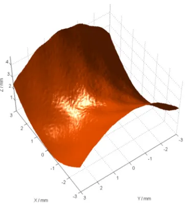
Two freeform surface case studies are employed to illustrate the capabilities of the proposed computation theory for morphological filters. In Figure 14, a saddle surface is presented with a number of tiny bump features on the surface topography. It can also be observed that the surface has several twisted waves superimposed on the topography. Morphological symmetrical filters (closing followed by opening) are applied to this surface with ball radius 0.5 mm and 2 mm respectively. Figure 15 illustrates the generated surfaces. It is obvious that bump features are suppressed by the filter in Figure 15(a) and wave features are also smoothed in Figure 15(b). By comparing the three surfaces, these topographical features of the surface can be separated and analysed.

[image:16.595.89.509.225.347.2]

[image:17.595.205.386.79.278.2]

Figure 14. An experimental saddle surface.

Figure 15. The smoothed surfaces generated by the application of morphological alternating symmetrical filters with ball radii: (a) 0.5 mm; (b) 2 mm.

[image:17.595.93.473.311.515.2] [image:17.595.212.374.566.746.2]

Figure 17. The envelope surface and residual surface generated by the application of morphological closing filter with ball radius 2.5 mm: (a) envelope surface; (b) residual surface.

7. Conclusion and future work

Morphological filters are useful tools in the surface analysis toolbox. Regarded as the complement to the mean-line based filtration techniques, morphological filters are relevant to the functional performance of surfaces, especially contact phenomenon of two mating surfaces. The conventional implementation of morphological filters has several fatal deficiencies that restrict the prevalence of morphological filters.

A full set of geometric computation theory for morphological filters is developed. On the basis of the relationship between the alpha hull and morphological envelopes, alpha shape theory is applied to the computation of morphological filters. The geometrical computation method brings in prominent capabilities so that the new algorithm works for freeform surfaces and suits non-uniform sampled surfaces, with arbitrary disk/ball radius enabled. The divide and conquer optimisation further improved the performance of the alpha shape method and reduced the memory usage. To release the dependence of the alpha shape method on the Delaunay triangulation, a set of definitions and propositions for searching contact points is presented and mathematically proved based on alpha shape theory. The contact point searching method is applicable to both circular and horizontal flat structuring elements, bringing in more generality over the alpha shape method.

Key issues of the future work include further improvement of the alpha shape algorithm by practical programming and efficient data structures, and further optimisation of the contact point searching algorithm, which consists two aspects: (1) improve the performance. Recursion should be replaced by iteration to avoid the huge cost of stack manipulations; (2) improve the robustness against arbitrary and complex shapes of surfaces.

Acknowledgement

[image:18.595.118.473.73.272.2]

References

Barber, C. B., Dobkin, D. P. & Huhdanpaa, H. T. 1996 The Quickhull Algorithm for Convex Hulls. ACM T. Math. Software 4, 469-483. (doi: 10.1145/235815.235821)

Bernardini, F., Mittleman, J., Rushmeier, H., Silva, C. & Taubin, G. 1999 The ball-pivoting algorithm for surface reconstruction. IEEE T. Vis. Comput. Gr. 5, 349-359.

(doi:10.1109/2945.817351)

Bruzzone A. A. G., Costa H. L., Lonardo P. M. & Lucca D. A. 2008 Advances in Engineered Surfaces for Functional Performance. CIRP Ann. Manuf. Technol. 57, 750-769.

(doi:10.1016/j.cirp.2008.09.003)

Cormen, T. H., Leiserson C. E. & Rivest R. L. 1989 Introduction to Algorithms. US: The MIT Press.

Dietzsch, M., Gerlach, M. & Groger, S. 2008 Back to the envelope system with morphological operations for the evaluation of surfaces. Wear 264, 411-415. (doi:10.1016/j.wear.2006.08.042)

Edelsbrunner, H. & Mucke, E. P. 1994 Three-dimensional alpha shapes, ACM T. Graphic 13, 43-72. (doi: 10.1145/174462.156635)

Fischer, K. 2000 Introduction to Alpha Shapes,

http://www.inf.ethz.ch/personal/fischerk/pubs/as.pdf.

Goto, T., Miyakura, J., Umeda, K., Kadowaki, S., Yanagi K. 2005 A robust spline filter on the basis of L2-norm. Precis. Eng. 29,157-161. (doi:10.1016/j.precisioneng.2004.06.004) ISO 16610-40: 2010 Geometrical Product Specification (GPS)-Filtration, Part 40:

Morphological profile filters Basic concepts, Switzerland.

ISO 17450-1: 2011 Geometrical Product Specification (GPS)-General concepts, Part 1: Model for geometrical specification and verification, Switzerland.

Jiang, X. 2009 The evolution of surfaces and their measurement, The 9th International Symposium on Measurement Technology and Intelligent Instruments, 54-60.

Jiang X., Lou, S. & Scott, P. J. 2012 Morphological Method for Surface Metrology and Dimensional Metrology Based on the Alpha Shape, Meas. Sci. Technol. 23, 015003. (doi:10.1088/0957-0233/23/1/015003)

Jiang, X., Copper, P. & Scott, P. J. 2011 Freeform surface filtering using the diffusion equation, Proc. R. Soc. A, 467, 841-859. (doi:10.1098/rspa.2010.0307)

Jiang, X., Scott, P. J., Whitehouse, D. J. & Blunt, L. 2007 Paradigm shifts in surface metrology, Part II. The current shift. Proc. R. Soc. A. 463, 2071-2099.

(doi:10.1098/rspa.2007.1873)

Jiang, X. & Whitehouse, D. J. 2012 Technological shifts in surface metrology, CIRP Ann. Manuf. Technol. 61:815-836. (doi:10.1016/j.cirp.2012.05.009)

Krystek, M, 1996 Form filtering by splines. Measurement 18, 9-15. (doi: 10.1016/0263-2241(96)00039-5)

Kumar, J. & Shunmugam M. S. 2006 A new approach for filtering of surface profiles using morphological operations. Int. J. Mach. Tools Manuf. 46, 260-270. (doi:

10.1016/j.ijmachtools.2005.05.025)

Peklenik, J. 1973 Envelope characteristics of machined surfaces and their functional importance. Proceedings of the Conference on Surface Technology, 74-95.

Peters, J., Bryan, J. B., Eslter, W. T., Evans, C., Kunzmann, H., Lucca, D. A., et al 2001 Contribution of CIRP to the development of metrology and surface quality evaluation during the last fifty years. CIRP Ann. Manuf. Technol. 50 (2), 471-488. (doi:

10.1016/S0007-8506(07)62996-5)

Peters, J., Vanherck, P. & Sastrodinoto, M. 1979 Assessment of surface typology analysis techniques. CIRP Ann. Manuf. Technol. 2, 1-25.

Radhakrishnan, V. & Weckenmann, A. 1998 A close look at the rough terrain of the surface finish assessment. P. I. Mech. Eng. B-J. Eng. 212, 411-420.

(doi:10.1243/0954405981516012)

Sayles, R. S. 2001 How two- and three-dimensional surface metrology data are being used to improve the tribological performance and life of some common machine elements. Tribol. Int. 34, 299-355. (doi: 10.1016/S0301-679X(00)00121-3)

Scott, P. J. 1992 The mathematics of motif combination and their use for functional

simulation. Int. J. Mach. Tools Manufact. 32: 69-73. (doi:10.1016/0890-6955(92)90062-L) Scott, P. J. 2000 Scale-space techniques. Proceedings of the X International Colloquium on

Surfaces, 153-161.

Seewig, J. 2006 Linear and robust Gaussian regression filters. J. Phys.: Conf. Ser. 13, 254-257. (doi:10.1088/1742-6596/13/1/059)

Serra, J. 1982 Image Analysis and Mathematical Morphology, New York: Academic Press. Shunmugam, M. S. & Radhakrishnan, V. 1974 Two-and three dimensional analyses of

surfaces according to the E-system. P. I. Mech. Eng. B-J. Eng. 188, 691-699. (doi:10.1243/PIME_PROC_1974_188_082_02)

Srinivasan, V. 1998 Discrete morphological filters for metrology. Proceedings of the 6th ISMQC Symposium on Metrology for Quality Control in Production, 623-628.

Tholath, J. & Radhakrishnan, V. 1999 Three-dimensional filtering of engineering surfaces using envelope system. Precis. Eng. 23, 221-228. (doi:10.1016/S0141-6359(98)00027-0) Thomas, T.R. 1999 Rough Surfaces. London, UK: Imperial College Press.

Trumpold, H. 2001 Process related assessment and supervision of surface textures. Int. J. Mach. Tools Manufact. 41, 1981-1993. (doi:10.1016/S0890-6955(01)00062-1)

Unswoth, A. 1995 Recent developments in the tribology of artificial joints. Tribol. Int. 28, 485-495. (doi:10.1016/0301-679X(95)00027-2)

Von Weingraber, H. 1956 U¨ ber die Eignung des Hu¨llprofils als Bezugslinie f¨ur die Messung der Rauheit, CIRP Ann. Manuf. Technol. 5, 116-128.

Westberg, J. 1997 Opportunities and problems when standardising and implementing Surface Structure parameters in Industry. Int. J. Mach. Tools Manufact. 38, 413-416.

(doi:10.1016/S0890-6955(98)00004-2)

Whitehouse, D. J. 1978 Surfaces- a link between manufacture and function. P. I. Mech. Eng. B-J. Eng. 192, 179-188. (doi: 10.1243/PIME_PROC_1978_192_018_02)

Whitehouse, D.J. 2001 Function maps and the role surfaces. Int. J. Mach. Tools Manufact. 41, 1847-1861. (doi:10.1016/S0890-6955(01)00049-9)

Whitehouse, D. J. 2002 Surfaces and their Measurement. UK: Hermes Penton Ltd. Whitehouse, D. J. & Reason, R. E. 1965 The equation of the mean line of surface texture

found by an electric wave filter, UK: Rank Taylor Hobson.

Worring, M. & Smelders, W. M. 1994 Shape of arbitrary finite point set in R2, J. Math. Imaging Vision. 4: 151-170. (doi: 10.1007/BF01249894)

Zeng, W., Jiang, X. & Scott, P. J. 2010 Fast algorithm of the Robust Gaussian Regression Filter for Areal Surface Analysis. Meas. Sci. Technol. 21, 055108. (doi:10.1088/0957-0233/21/5/055108)