Real Time Bayesian Analysis of Ground Motion Envelopes for Earthquake Early Warning

(1)

for

Earthquake Early Warning

Thesis by

Gokcan Karakus

In Partial Fulfillment of the Requirements

for the Degree of

Doctor of Philosophy

California Institute of Technology

Pasadena, California

2016

(2)

Gokcan Karakus

(3)

Acknowledgements

I would like to thank my advisor, Prof. Thomas H. Heaton, for his extremely

helpful advice and limitless patience towards me everyday, without exception, during our

collaboration. I feel tremendous honor to be his student.

I would like to thank Prof. James L. Beck for his very important help on the

statistical portion of my research. I could not have achieved it without you; thank you.

Starting with Prof. Jean Paul Ampuero, I would like to thank my PhD examining

committee. It has been my honor to have him, Prof. Hiroo Kanamori and Prof. Domniki

Asimaki on my PhD examining committee.

Starting with Dr. In Ho Cho, I would like to thank the students of Civil

Engineering option at Caltech for their company and help during my stay at Caltech.

Starting with Dr. Arthur Lipstein, I would like to thank my friends at Caltech who

were associated with options other than Civil Engineering.

Starting with Carolina Oseguera, I would like to thank the staff of the Civil

Engineering option at Caltech for creating a positive work environment for me.

Starting with Dr. Yannik Daniel Behr, Dr. Men-Andrin Meier and Dr. Maren

Boese, I would like to thank my colleagues at institutions different from Caltech for their

help and support.

Starting with the International Student Program (ISP), I would like to thank all of

the offices and staff at Caltech for doing their job so well so that I could focus on my

(4)

Starting with Prof. Cem Yalcin, I would like to thank the civil engineering faculty

in my undergraduate institution, Bogazici University, who helped me prepare for a

journey of lifelong learning.

I would like to especially thank Dr. Georgia B. Cua for her constant help, and for

starting an envelope based earthquake early warning method.

And, finally, I would like to thank my family in Turkey for their emotional

(5)

Abstract

Current earthquake early warning systems usually make magnitude and location

predictions and send out a warning to the users based on those predictions. We describe

an algorithm that assesses the validity of the predictions in real-time. Our algorithm

monitors the envelopes of horizontal and vertical acceleration, velocity, and

displacement. We compare the observed envelopes with the ones predicted by Cua &

Heaton’s envelope ground motion prediction equations (Cua 2005). We define a “test

function” as the logarithm of the ratio between observed and predicted envelopes at every

second in real-time. Once the envelopes deviate beyond an acceptable threshold, we

declare a misfit. Kurtosis and skewness of a time evolving test function are used to

rapidly identify a misfit. Real-time kurtosis and skewness calculations are also inputs to

both probabilistic (Logistic Regression and Bayesian Logistic Regression) and

nonprobabilistic (Least Squares and Linear Discriminant Analysis) models that ultimately

decide if there is an unacceptable level of misfit. This algorithm is designed to work at a

wide range of amplitude scales. When tested with synthetic and actual seismic signals

(6)

Chapter 3 Probabilistic Classifications ... 21

3.1 Classifications – Probabilistic Generative Model ... 22

3.2 Discussion of Results for Tables 3.1 to 3.3 ... 34

3.3 Classification – Probabilistic Discriminative Model with Maximum Likelihood Estimate (MLE) ... 34

(7)

3.5 Classification – Probabilistic Discriminative Model with Maximum A Posteriori

(MAP) Value ... 41

3.6 Discussion of Results in Table 3.7 to 3.9 ... 48

3.9 Classification – Posterior Predictive Distribution ... 56

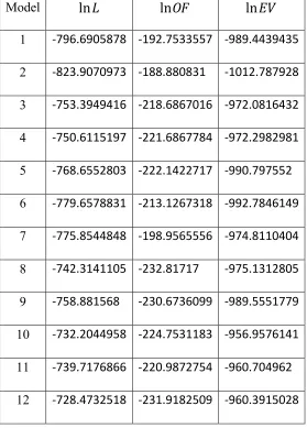
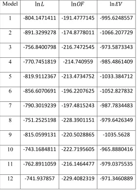
3.10 Classification – Bayesian Model Class Selection (Method I) ... 58

3.11 Classification – Sparse Bayesian Learning (Method II) ... 68

Chapter 4 Case Studies – Okay Predictions ... 75

4.1 Okay-Prediction Examples ... 76

4.1.1 Okay-prediction example 1 ... 76

4.1.2 Discussion of okay-prediction example 1 ... 77

4.1.3 Okay-prediction example 2 ... 84

4.1.4 Discussion of okay-prediction example 2 ... 84

4.1.5 Okay-prediction example 1 with arrival time perturbations ... 94

4.2 A Supplementary Method for the Reality Check Algorithm ... 106

4.2.1 Karakus-Heaton Moment of Signal Data ... 108

Chapter 5 Case Studies – Over Predictions ... 118

5.1 Over-prediction example 1 ... 118

5.1.1 Discussion of over-prediction example 1 ... 126

5.2 Over-prediction example 1 with matching envelope arrival times ... 128

(8)

5.3 Over-prediction example 2 ... 134

5.3.1 Discussion of over-prediction example 2 ... 147

Chapter 6 Case Studies – Under Predictions ... 149

6.1 Discussion of under-prediction example ... 156

Chapter 7 Concluding Remarks and Future Work ... 158

Appendix A Virtual Seismologist Envelope Equations ... 162

Appendix B Multiple Window Approach ... 164

Appendix C Non-probabilistic Classifications ... 167

C.1 Classifications: Least Squares ... 167

C.2 Discussion of Results in Tables C.1 to C.3 ... 169

C.3 Classifications – Linear Discriminant Analysis (LDA) ... 174

C.4 Discussion of Results in Tables C.4 to C.6 ... 185

(9)

List of Figures

1.1 Schematic illustration of the reality check algorithm ………... 3

2.1 Example of an observed and a predicted envelope ……… 5

2.2 Examples of predicted envelopes generated using the Virtual Seismologist method ……… 7

2.3 Envelopes and their test function ………... 9

2.4 A test function result and its histogram ………... 10

2.5 Graphical interpretation of higher order statistics ………... 13

2.6 Example of a double event seismogram and its envelope ………... 14

2.7 Under-prediction, i.e., missed event example ……….. 16

2.8 Over-prediction, i.e., false alarm example ………... 18

2.9 Three states of the test function ………... 20

4.1 Reality Check Algorithm’s performance plot for the okay-prediction example 1 computed using (3.68) from acceleration input using Method I ……….. 78

4.2 Reality Check Algorithm’s performance plot for the okay-prediction example 1 computed using (3.69) from velocity input using Method I ……….... 79

4.3 Reality Check Algorithm’s performance plot for the okay-prediction example 1 computed using (3.70) from displacement input using Method I ……….... 80

4.4 Reality Check Algorithm’s performance plot for the okay-prediction example 1 computed using (3.99) from acceleration input using Method II ……… 81

(10)

4.6 Reality Check Algorithm’s performance plot for the okay-prediction example 1

computed using (3.101) from displacement input using Method II ………. 83

computed using (3.68) from acceleration input using Method I ……….. 85

computed using (3.69) from velocity input using Method I ……….... 86

computed using (3.70) from displacement input using Method I ……….... 87

computed using (3.99) from acceleration input using Method II ……… 88

computed using (3.100) from velocity input using Method II ………. 89

computed using (3.101) from displacement input using Method II ………. 90

computed using (3.101) from displacement input using Method II (zoomed-in on

the first over-prediction indication) ………. 92

computed using (3.101) from displacement input using Method II (zoomed-in on

the second over-prediction indication) ………. 93

(11)

(with early predicted P-wave arrival) computed using (3.99) from acceleration

input using Method II ………... 96

(with early predicted P-wave arrival) computed using (3.100) from velocity input

using Method II ……… 98

(with early predicted P-wave arrival) computed using (3.101) from displacement

input using Method II ………... 99

(with early predicted P-wave arrival) computed using (3.100) from velocity input

using Method II (zoomed-in on the early predicted P-wave arrival) …………. 100

(with late predicted P-wave arrival) computed using (3.99) from acceleration

input using Method II ………. 101

(with late predicted P-wave arrival) computed using (3.100) from velocity input

using Method II ……….. 102

(with late predicted P-wave arrival) computed using (3.101) from displacement

(12)

(with late predicted P-wave arrival) computed using (3.101) from displacement

input using Method II (zoomed-in on the late predicted P-wave arrival) …….. 104

4.24 Static moment computation illustration in 2D ………... 110

4.25 Comparison of taking logarithm with applying Karakus-Heaton Moment of Signal

Data ……… 113

4.26 Performance of the supplementary method to RCA for the okay-prediction

example 1 ………... 115

example 1 (with early predicted P-wave arrival) ………... 116

example 1 (with late predicted P-wave arrival) ………. 117

5.1 Summary of July 1st 2015 false alarms ……….. 119

5.2 Reality Check Algorithm’s performance plot for the over-prediction example 1

(with predicted wave arriving earlier than observed calibration pulse) computed

using (3.99) from acceleration input using Method II ………... 122

using (3.100) from velocity input using Method II ……… 123

(13)

5.5 Performance of the supplementary method to RCA for the over-prediction

example 1 (with predicted wave arriving earlier than observed calibration pulse)

125

using (3.99) from acceleration input using Method II (zoomed-in at arrival times

of observed and predicted envelopes) ……… 127

(with predicted wave arriving at the same time as observed calibration pulse)

computed using (3.99) from acceleration input using Method II ……….. 129

computed using (3.100) from velocity input using Method II ………... 130

computed using (3.101) from displacement input using Method II …………... 131

example 1 (with predicted wave arriving at the same time as observed calibration

(14)

computed using (3.99) from acceleration input using Method II (zoomed-in at

arrival times of observed and predicted envelopes) ………... 135

computed using (3.101) from displacement input using Method II (zoomed-in at

arrival times of observed and predicted envelopes) ………... 136

5.13 Seismic data for the calibration pulse that is used as an over-prediction example 1

from the Northern California Earthquake Data Center ……….. 137

5.14 Seismic data for the calibration pulse that is used as an over-prediction example 1

from the Northern California Earthquake Data Center, zoomed-in around missing

data ………. 138

(15)

computed using (3.99) from acceleration input using Method II with matching

arrival times of observed abnormal noise increase and predicted P-wave …… 143

computed using (3.100) from velocity input using Method II with matching

computed using (3.101) from displacement input using Method II with matching

example 2 with matching arrival times of observed abnormal noise increase and

predicted P-wave ……… 146

6.1 Reality Check Algorithm’s performance plot for the under-prediction example

6.4 Performance of the supplementary method to RCA for the under-prediction

(16)

computed using (3.99) from acceleration input using Method II (zoomed-in at

arrival time of the small preceding event in the seismogram, and Cucapah – El

Mayor earthquake in ground motion envelopes) ………... 155

B.1 Kurtosis computation example with a single window of length 20 seconds …. 165

B.2 Multiple windows approach for a kurtosis computation with two different window

lengths and their sum ………. 166

C.1 Histogram for all three classes obtained using LDA with acceleration values only

177

C.2 Histogram for all three classes obtained using LDA with velocity values only 180

C.3 Histogram for all three classes obtained using LDA with displacement values only

(17)

List of Tables

3.1 Confusion matrix for probabilistic generative classification using acceleration

data ………... 29

3.2 Confusion matrix for probabilistic generative classification using velocity data

31

3.3 Confusion matrix for probabilistic generative classification using displacement

data ………... 33

3.4 Confusion matrix for probabilistic discriminative classification with MLE using

acceleration data ………... 38

velocity data ………... 39

displacement data ………... 40

3.7 Confusion matrix for probabilistic discriminative classification with MAP

(_!σ =100) using acceleration data ………... 45

(_!σ =100) using velocity data ……….. 46

(_!σ =100) using displacement ………... 47

(_!σ =10) using acceleration data ……….. 49

(18)

(_!σ =10) using displacement data ……….... 51

3.13 Confusion matrix for probabilistic discriminative classification with MAP (_!σ =0.05) using acceleration data ………... 53

3.14 Confusion matrix for probabilistic discriminative classification with MAP (_!σ =0.05) using velocity data ………... 54

3.15 Confusion matrix for probabilistic discriminative classification with MAP (_!σ =0.05) using displacement data ………... 55

3.16 List of features included in alternative models ……… 64

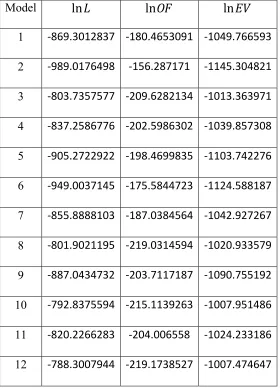
3.17 Bayesian model class selection results for acceleration input ………... 65

3.18 Bayesian model class selection results for velocity input ……… 66

3.19 Bayesian model class selection results for displacement input ………... 67

C.1 Confusion matrices for least squares classification using acceleration data ….. 171

C.2 Confusion matrices for least squares classification using velocity data ……… 172

C.3 Confusion matrices for least squares classification using displacement data … 173 C.4 Confusion matrix for LDA using acceleration data ………... 178

C.5 Confusion matrix for LDA using velocity data ………. 181

(19)

Chapter 1

Introduction

Recently, the earthquake early warning (EEW) systems are being developed in

many parts of the world. These systems do not predict when an earthquake is going to

happen; rather they predict the eventual characteristics of earthquakes, such as their

magnitude and location, by using the first few seconds of the earthquakes’ ground motion

data that are being recorded by seismic stations in real-time. Unfortunately, the seismic

stations records do not only contain earthquake data, but also any activity that “shakes”

the ground, such as sonic booms, quarry blasts, and even heavy traffic noise. These types

of activities may confuse a warning system that relies on ground motion amplitudes

recorded by seismograms being larger than certain thresholds. In addition to

non-earthquake activity, temporal distribution of actual non-earthquakes, such as an non-earthquake

swarm instead of an isolated earthquake being preceded and followed by quiet ground

motion periods, may affect the accuracy of the alert messages sent to the EEW system

subscribers.

The current EEW system being tested in California does not have a mechanism

that checks the accuracy of the messages sent to the system subscribers. However, we

desire to have a sophisticated real-time checking mechanism that will oversee and verify

the system predictions. To develop a robust alert confirmation mechanism, we examined

more than 500 synthetically created false and missed EEW alert scenarios for earthquakes

(20)

We used earthquake waveform envelope data predicted by Cua & Heaton’s

envelope ground motion prediction equations (Cua 2005) to verify the predictions made

by the EEW system. During the comparison calculations between observed and predicted

ground motions, we measured the disagreement using higher order statistics: kurtosis and

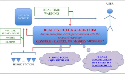
skewness. We developed a new algorithm called reality check (Figure 1) that classifies

the state of an EEW system alert based on the kurtosis and skewness measures of the

misfit between observed and predicted waveform envelope data.

This thesis presents the step-by-step development process of the reality check

algorithm and shows how this technique helps protect the credibility of an EEW system

(21)

[image:21.612.110.543.71.330.2]

Figure 1.1: Schematic illustration of the reality check algorithm. The recorded ground motion data are sent to a main computer called Decision Module. Decision Module

makes a prediction using several algorithms (Virtual Seismologist, Onsite, and Elarms)

and sends an alert to the users if necessary. The Reality check algorithm receives the sent

alert messages, and then compares them with the real-time recorded data by seismic

stations and reports the accuracy of the messages back to the decision module. We

(22)

Chapter 2

Data Processing

2.1 Data Processing

This section describes the choice of input used regarding the ground motion data.

The seismic stations in California can record ground motion in from 80 samples

per second (broadband seismometers) to 100 samples per second (strong motion

seismometers). Our algorithm does not use these recordings directly. Instead, we use

envelopes of the waveform data. We run a 1 second long window throughout the

continuous records in real-time, and take the absolute maximum value within the window

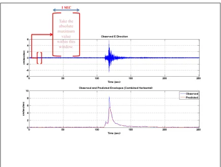
and make it our envelope amplitude at the corresponding second in real-time (Figure 2.1).

Then, we slide the window to the next second and so on. This process gives us the

“envelope of the observed data” whether there is an event or just noise at a site.

2.2 Prelude: Virtual Seismologist

The Virtual Seismologist (VS) (Cua 2005) is briefly explained in this section,

because it is a prerequisite for our algorithm.

Our work uses envelopes of earthquake waveform data rather than the

seismogram recordings directly as explained in the previous section. In addition to the

observed earthquake envelopes, we make use of predicted envelopes that are created by

the ground motion prediction equations provided by the Virtual Seismologist. The Virtual

Seismologist (VS) (Cua 2005) was developed at Caltech. It is a Bayesian Inference

Framework based on waveform envelopes and prior information, e.g., foreshocks,

(23)

[image:23.612.109.544.68.397.2]

Figure 2.1: Example of an observed and a predicted envelope. Plot on top shows a broadband seismogram recorded at 80 samples per second rate at a station in E-W

direction. We run a 1 second long window throughout the continuous records in

real-time, and take the absolute maximum value within the window and make it our envelope

amplitude at the corresponding second in real-time. Note that the envelope shown in blue

in the bottom plot is a combination on E-W and N-S horizontal envelopes. Note that the

bottom plot also shows the corresponding predicted envelope created using the Virtual

Seismologist method.

1 SEC

Take the absolute maximum

value within this

(24)

waveform envelopes as a function of amplitude and distance. We need to provide the

magnitude ofthe event and the distance between its epicenter and a particular station to

create the estimated envelopes at that station. In addition to the P- and S-wave envelopes,

VS predicted envelopes also contain a constant noise envelope that represents the noise

level at a particular station. These three envelopes (P-wave, S-wave, and constant noise)

are combined in a square root of sum of squares fashion to produce the VS predicted

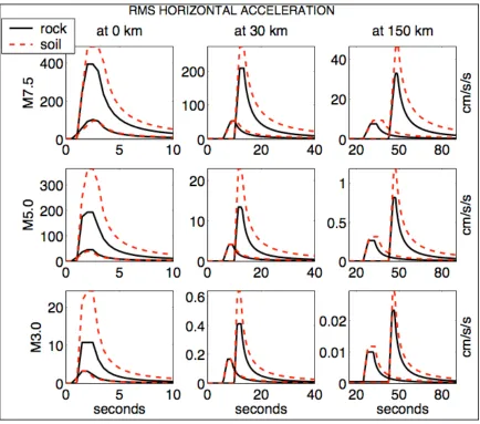
envelopes at a given station for a given earthquake. Examples of VS predicted envelopes

are shown in Figure 2.2.

!VS!Envelope!=! P-wave!Envelope

(

)

2

+

(

S-wave!Envelope

)

2+

(

Noise!Envelope

)

2 (2.1)

The data for this work are collected from Southern California Seismic Network (SCSN)

and Next Generation Attenuation (NGA) strong motion data. Figure 2.2 shows examples

of predicted envelopes generated using the Virtual Seismologist method. VS equations

for predicting envelopes are given in Appendix A.

2.3 Test Functions

This section explains what we do right after we obtain both the observed and

predicted envelopes. Because the seismic stations continuously record ground motions

and we assume there will always be some noise being recorded at a station, the predicted

envelope (2.1) only consists of constant noise when the decision module is not publishing

any earthquake data. That means we have both observed and predicted envelope data at

any given time. Therefore, the following steps are performed at every second in real-time.

Once we have both predicted and observed envelope values, we calculate the

(25)

Figure 2.2: Examples of predicted envelopes generated using the Virtual Seismologist method. Note that there is a binary classification as soil/rock at station sites. A different

set of ground motion prediction equations are provided for each site class by VS.

[image:25.612.110.544.70.453.2]

(26)

! !

φ

( )

nΔt =B_HP∗log Observed!Envelope

( )

nΔt Predicted!Envelope

( )

nΔt

⎛ ⎝

⎜⎜ ⎞_⎠⎟⎟ (2.2)

where

= 1,2,…

: envelope sampling rate (1 second)

: convolution symbol

: Butterworth high-pass filter, 2nd_{order, 600 seconds, see below for justification.}

: test function

Test functions, denoted , are second by second misfit computations between observed

and predicted envelopes. Figure 2.3 shows that a test function represents the time

evolution of the misfit between observed and predicted ground motion values.

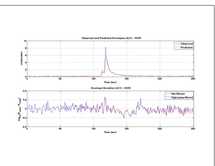
In some of our calculations, we noticed that the misfit in the S-wave coda is

usually different from the rest of the misfit, especially for the displacement misfit, if we

do not apply high-pass filtering to the ratio of logarithm of envelope values (Figure 2.3).

In order not to confuse our algorithm, which indirectly depends on the amplitude of the

misfit, we decided to high-pass filter the ratios between observed and predicted ground

motion values. We apply a recursive high-pass Butterworth filter to the raw misfit.

2.4 Virtual Seismologist Assumption Regarding Misfit

The data fitting process in creating the predicted envelope GMPE’s was done by

modeling the difference between predicted and observed ground motion envelopes as a

Gaussian distribution with a mean of zero in logarithm space. This model was chosen by

the VS creators and we should check how well it does. The histogram of the test function

results from the previous example is shown in Figure 2.4.

!n

!Δt

∗

!BHP

φ

(27)

Figure 2.3: Envelopes and their test function. (On top) The observed and predicted envelopes shown in Figure 2.1. (On bottom) Test function computed using (2.2) both

[image:27.612.112.544.63.398.2]

(28)

[image:28.612.112.545.68.396.2]

(29)

Each one of the bins shown at the bottom of Figure 2.4 represents an amplitude value in

the graph above. All of the values of the test function are distributed about the mean as

shown in the histogram, and a Gaussian (_!µ =−0.0104,σ =0.0718) distribution is

adequate to explain it. The VS regression analysis included more than 30,000

seismograms, so this much departure from normality in one example is within acceptable

limits (this is not based on an analysis, it is just a qualitative judgment). The assumption

is observed to be valid.

It is relatively easy for a human to visually notice if a distribution departs from a

Gaussian one, but how can we make a computer detect any unacceptable departure

automatically in real-time? One answer is to use higher order statistics: kurtosis and

skewness.

2.5 Higher Order Statistics

We use higher order statistics to detect departure from normality. Using higher

order statistics makes these techniques more robust than just using the mean and the

standard deviation.

2.5.1 Higher Order Statistics – Kurtosis

Kurtosis is a normalized fourth moment of a distribution about its mean where the

normalization is done using the square of the variance (Langet, Maggi et al. 2014), so it

does not have a unit. It is mainly used to detect outliers based on a normal distribution.

Kurtosis for a normal distribution is the value three (3), so outliers in the tails of the

(30)

(2.3)

where

: expected value

: set of values in a distribution

: mean of the set of values in

2.5.2 Higher Order Statistics – Skewness

Skewness, on the other hand, is the third moment about the mean of a distribution,

and just like kurtosis, it is normalized using the appropriate power of the variance, so

skewness too is dimensionless. Skewness is used to detect departure from symmetry. Its

sign depends on the direction of the skew as shown in Figure 2.5. A normal distribution is

perfectly symmetric about its mean and so its skewness is zero.

(2.4)

Note that higher order statistics equations, i.e., (2.3) and (2.4) are for theoretical moments

and they must be replaced by sample moments when applied to data. Matlab functions

‘kurtosis’ and ‘skewness’ are used on the data, however, ‘bias correction’, as explained in

the function definition in Matlab, was not applied.

! !

Kurtosis= E X

(

−µ

)

4 ⎡

⎣⎢ ⎤⎦⎥

E X⎡

(

−µ

)

2 ⎣⎢ ⎤⎦⎥ ⎛ ⎝⎜ ⎞⎠⎟ 2 !E !X µ _!X ! !

Skewness= E X

(

−µ

)

3 ⎡

⎣⎢ ⎤⎦⎥

E X⎡

(

−µ

)

2 ⎣⎢ ⎤⎦⎥ ⎛

⎝⎜ ⎞⎠⎟

(31)

2.6 An Example – Missed Event

We now take a look at an example and see the algorithm in action. The following

example aims to simulate an ‘under-prediction’ case where the system misses an event. In

order to emphasize an under-prediction case, the following figure also includes a case

where the system successfully detects an earthquake, i.e., the first one (Figure 2.6). The

top of Figure 2.6 shows a synthetic seismogram. We basically put two identical events

Figure 2.5: Graphical interpretation of higher order statistics.

KURTOSIS FOR A

NORMAL

DISTRIBUTION IS 3.

OUTLIERS IN “TAILS”

OF A DISTRIBUTION

CAUSE POSITIVE

KURTOSIS

(i.e. KURTOSIS >>3).

SKEWNESS FOR A

NORMAL

DISTRIBUTION IS 0.

“ASYMMETRY”

CAUSES NON-ZERO

(32)

Figure 2.6: Example of a double event seismogram and its envelope. (On top) seismogram, (on bottom) envelope. Envelopes on the bottom are two horizontal

(33)

(~M4.6) back to back in time. On the bottom of Figure 2.6, we see the envelopes created

using the technique demonstrated earlier. From now on, we will not show the

seismogram itself, and we will work with the envelopes instead.

In this scenario (Figure 2.7), incoming data from the first event stimulated the

system to the point where an alarm is issued. The magnitude and the location of the event

related to the first alarm are used to create the VS envelopes and they are overlaid on top

of the observed ones using the origin time predicted by the decision module. However,

there happens to be a second event and the system does not catch it. We calculate our test

function in real-time as more data are recorded. Then, time derivatives of kurtosis and

skewness, which are computed using a multiple window approach (see Appendix B) on

the test function values, are computed in real-time as well.

Everything seems fine until the second event arrives at the station. In other words,

both derivative of excess kurtosis and derivative of skewness values indicate normality;

therefore, there is agreement between the decision module alert and what is actually

observed. But, once the second event arrives, the test function shows values that are

considered as outliers and this produces significantly greater values of the derivatives.

Moreover, because the symmetry is lost, derivative of skewness values indicate positive

skew.

2.7 Another Example – False Event

With an example of a false alarm case, we now show some justification for using

two higher order statistics functions instead of one. Kurtosis would give us a very large

number if we had a false alarm. That is, if the corresponding test function value was a

(34)

(35)

computed by using equation (2.2), it would be considered as an outlier, similar to the case

of missed alarm example. In other words, as far as kurtosis is concerned, there is no

difference between the outliers on the left or on the right tail of the mean. However,

skewness would detect a negative skew in that scenario (Figure 2.8), and we would know

the “nature” of the departure from normality. That is why we use both kurtosis and

skewness in our algorithm.

In the scenario shown in Figure 2.8, the decision module predicts an earthquake,

and issues the parameters that are needed to create the VS predicted envelopes. All is

well. After the earthquake, however, the station that recorded this seismogram

experiences some non-earthquake shaking in the form of a short lasting burst of energy,

for example, traffic noise nearby. This blip seen in the top row tricks the decision module

to issue another alarm, then our algorithm creates the corresponding VS envelope and

starts measuring the agreement between the observed and predicted envelopes. As soon

as the unacceptable mismatch is detected with the help of derivative of higher order

statistics, our algorithm indicates an over-prediction.

2.8 Summary of Test Function States

To sum up, we declare that there are three states that a test function can be in

(Figure 2.9):

State 1: The ideal case where the decision module reports agreement with the

observed data, i.e., okay-prediction.

State 2: There is a second event when we thought there was only one, i.e.,

(36)

(37)

State 3: A non-earthquake vibration such as noise at a station tricks the system

into believing that there is an earthquake, i.e., false event/alarm. This one is especially

tricky because one might lose confidence in the warning system.

We perform separate analyses for different ground motion parameters influenced

by different frequency contents; acceleration, velocity, and displacement are separately

used as inputs to our computations. We obtained our training data by synthetically

creating over- and under- prediction scenarios. The VS predicted envelopes were created

using the cataloged magnitude and location. Our training data included 1000

okay-prediction, 250 over-okay-prediction, and 250 under-prediction input values in both horizontal

and vertical acceleration, velocity, and displacement.

The peak values of derivatives of kurtosis and skewness for both horizontal and

vertical acceleration, velocity, and displacement, at the moment of unacceptable

mismatch between observed and predicted envelopes as shown in the figures above, are

considered as inputs that belong to under- and over- prediction classes: under-prediction

if observed envelope value is significantly larger, and over-prediction if predicted

envelope value is significantly larger. Maximum and minimum values of the derivatives

preceding the peak values mentioned above are considered as inputs of the

okay-predictions because they represent the boundaries within which the state of the prediction

is acceptable. We use these values as inputs for various classification models explained in

the following sections. Note that the coefficient values presented in this thesis are

truncated versions although they are used, in computations, as the computer programs

produced, i.e. with higher precision. We used our judgment regarding meaningful

(38)

Figure 2.9: Three states of the test function.

•  STATE 1: ϕ ≈ 0 (i.e. Agreement between envelopes)

•  STATE 2: ϕ >> 0 (i.e. Under prediction)

•  STATE 3: ϕ << 0 (i.e. Over prediction)

We use Linear Discriminant and Bayesian Analyses to classify the states at every second in real-time by minimizing the overlapped areas.

Env(obs) << Env(pred)

Kurtosis >> 3

Skewness << 0 Env(obs) >> Env(pred)

Kurtosis >> 3

Skewness >> 0

Env(obs) ≈ Env(pred)

Kurtosis ≈ 3

Skewness ≈ 0

MISSED OK FALSE

State 1

(39)

Chapter 3

Probabilistic Classifications

Mathematical Notation:

Throughout this work, unless stated otherwise, we use lowercase bold Roman

letters, such as , to denote vectors. All vectors are assumed to be column vectors.

Therefore is a -dimensional vector. We use uppercase bold Roman

letters, such as , to denote matrices.

Classifications:

In the following sections, we present different ways of applying classification.

Two probabilistic classification methods are described in this chapter (towards the end of

it): Method I which uses Ockham’s razor on a given set of models, and Method II which

uses Sparse Bayesian Learning (SBL), i.e., models with Automatic Relevance

Determination (ARD) prior. Note that both of these methods are using Bayesian Ockham

razor by maximizing evidence (or posterior probability); with ARD prior, it is a

continuum of model classes, each defined by specifying hyperparameters (prior

variances), instead of a discrete set of model classes (personal communication with Prof.

James L Beck). Two non-probabilistic classification methods were also examined: least

squares and linear discriminant analysis. The theory and results for these

non-probabilistic methods are presented in Appendix C. Appendix C is included for two main

purposes: 1) to provide classification methods that do not require as much run time as the

!x

! !

!x=⎡⎣x1,x2,,xD⎤⎦ T

!D

(40)

probabilistic methods, 2) to help some interested readers understand probabilistic

classification models if classification is a new concept to them.

We aim to have the least amount of misclassification rate when we take an input

vector and assign it to a class among discrete classes. Unless it is specified

otherwise, we will use linear models where the decision boundaries that separate classes

are linear functions of the input. The number of classes in our work is three, i.e.,

(Figure 2.9). We will use a coding scheme (as described in Bishop, 2006) in

which the target vector is of length such that if the class for an input is , then

all elements of are zero except element , which takes the value 1 (Bishop 2006).

Our classifications will generally be done using a discriminant function. The parameters

of the discriminant functions are obtained with several different techniques in the

following sections.

3.1 Classifications – Probabilistic Generative Model

The following theory is based on the concepts described in Chapter 4, Linear

Models for Classification in Bishop, 2006.

In this chapter, we work with Bayesian probabilistic classifications so when a new

input is observed, we compute probability (the degree of plausibility) that it belongs to

any class.

We start with generative models. Generative models use a probability model for

the inputs and outputs; that is, we can create synthetic input data by sampling from the

generative probabilistic model. In this section, we aim to compute posterior probabilities,

!x !K

!

!K=3

!

!1−of −K

!t !!K =3 _!Cj

(41)

!

!p C

( )

k x , with the help of Bayes’ theorem. In order to do that, we model both

class-conditional densities !

!p

( )

xCk and class priors _!p C

( )

k .

Our classification problem has three classes. In practice, the problems with more

than two classes, i.e., !!K >2 are considered “multiclass” classification problems. It is

common to use a softmax function in a multiclass classification problem. So, to better

understand what a softmax function represents, let us start with a two-class classification

problem set up (_!_!K=2) and then try to generalize our computations to a multiclass

classification problem. If we had only two classes, i.e., _!_!C₁ and _!_!C₂ we could write the

posterior probability for class _!_!C₁ as

!

p C

( )

₁x = p

( )

xC1 p C

( )

1

p

( )

xC₁ p C

( )

₁ +p

( )

xC₂ p C

( )

₂ (3.1)

We can write (3.1) as

! !

!

p C

( )

₁ x =σ

( )

a = 1

1+exp

( )

−a (3.2)

where !a is implicitly defined as

!

a=lnp

( )

xC1 p C

( )

1

p

( )

xC₂ p C

( )

₂ (3.3)

and

!σ

( )

a defined by (3.2) is called the logistic sigmoid function. For a multiclass case

(where _!_!K>2), we consider _!a to be a linear function of the input _!x. From Bayes

(42)

!

p C

( )

_k x = p

( )

xCk p C

( )

k

p

( )

xC_j p C

( )

_j

j

∑

= exp

( )

ak exp

( )

a_j

j

∑

(3.4)

Expression (3.4) is known as the softmax function (or the normalized exponential). It is

regarded as a generalization of the logistic sigmoid to a multiclass problem. In this case,

the quantities _!a_k are defined as

!

!ak=ln

(

p

( )

xCk p C

( )

k

)

(3.5)

Let us now see what happens if we choose a Gaussian form for the

class-conditional densities

!

!p

( )

xCk . For simplicity, let us assume that all classes have the same

covariance matrix Σ but each class has a distinct mean _!_!m_k. Then, we can write the

class-conditional density for class _!C_k as

! ! !

p

( )

xC_k = 1

2π

( )

D/2

1

Σ1/2exp −

1

2 x

T₋_m

k

(

)

T

Σ−1 _xT₋_m

k

(

)

⎧ ⎨ ⎩ ⎫ ⎬

⎭ (3.6)

where _!D is the dimensionality of _!x. Using (3.4) and (3.5), we can write

!

!ak

( )

x =w

T_x₊_w

k0 (3.7)

where we used the following definitions

!

! !

w_k=Σ−1_m

k

w_k₀=−1

2mk T_Σ−1_m

k+lnp C

( )

k

(3.8)

Thanks to our assumption that all classes have the same covariance matrix, the quadratic

terms cancel and the !

(43)

boundaries being defined as linear functions of _!x, as opposed to the case where we do

not make the same covariance assumption. In that case (where each class has its own

covariance matrix), the quadratic terms would not cancel and we would no longer have a

linear discriminant.

In the next step, we will use maximum likelihood (maximum a posteriori for

uniform priors) to calculate the parameters,_!_!w_k and_!_!w_k₀, and the prior class probabilities,

!p C

( )

k . We have chosen a Gaussian form for class-conditional densities, _!_!p

( )

xCk , as we

mentioned above. We will use the data set described in Chapter 2; the training data set is

given as

!

{ }

xn,tn with !!n=1,,N. We construct !X with its !n

th_row

!

!xn

T_{given by an}

instance of ! ! ! x= d

dt

(

Kurtosis!of!Horizontal!Acceleration

)

d

dt

(

Kurtosis!of!Vertical!Acceleration

)

d

dt

(

Skewness!of!Horizontal!Acceleration

)

d

dt

(

Skewness!of!Vertical!Acceleration

)

⎡ ⎣ ⎢ ⎢ ⎢ ⎢ ⎢ ⎢ ⎢ ⎢ ⎢ ⎢ ⎤ ⎦ ⎥ ⎥ ⎥ ⎥ ⎥ ⎥ ⎥ ⎥ ⎥ ⎥ (3.9)

The target vector _!_!t_n is a binary vector of length _!_!K=3. It uses the _!_!1−of −K coding

scheme; it has components

!tnj=δjk (Kronecker delta) if input !n is from class !Ck. We denote the prior class probabilities as

(44)

We chose a probability model where the predictions of the features for class _!C_k

are independent, so the likelihood function is given by

! !

!p

(

T,Xπk,mk,Σ

)

=

{

p

( )

xnCk πk

}

t_nk

k=1 K

∏

n=1

N

∏

(3.11)

After taking the logarithm of (3.11), we get

!

!lnp

(

T,Xπk,mk,Σ

)

= k=1tnk

{

lnp

( )

xnCk +lnπk

}

K

∑

n=1

N

∑

(3.12)

To determine the prior probability for _!C_k, we take the derivative of (3.12) with respect to

!πk and equate it to zero, and note that _!_!

∑

kπk=1. Then we obtain

!πk = N_k

N (3.13)

where _!N_k represents the number of data points assigned to class _!C_k.

Let us next determine _!_!m_k. We will take the derivative of (3.12) with respect to

!

!mk and set the result to zero. Using (3.6) as the functional form of class-conditional

densities, we obtain

!

m_k = 1

N_k tnkxn

n=1 N

∑

(3.14)

which is simply the mean of all of the input vectors assigned to class _!C_k.

The only parameter left to determine is the shared covariance, Σ. Once again,

taking the derivative with respect to Σ and setting it to zero gives

! ! !Σ=

N_k N Sk k=1

K

∑

= π_kS_k

k=1

K

∑

(3.15)

(45)

!

! S_k= 1

N_k tnk

(

xn−mk

)

(

xn−mk

)

T

n=1

N

∑

(3.16)

Expressions (3.15) and (3.16) show that we can compute Σ by weighting the covariances of the data of each class by their prior probabilities and then averaging the result.

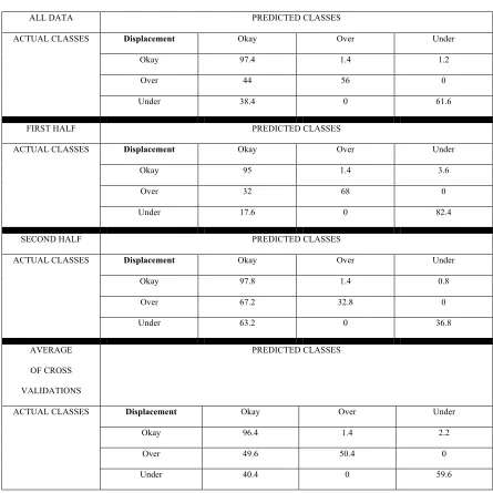
For the following confusion matrices (where the rows are the total percentage of a

labeled class, and hence the values in a row add up to 100, and the columns are the

fraction of the total number of cases for that row that is classified as the indicated class

on the top row of that column), we choose the maximum probability value for a given

input. Although the parameter values, _!_!w_k and _!_!w_k₀, are computed using the entire data

set for training, we provide confusion matrices for cross validation results for different

ground motion quantities. The confusion matrix is useful to assess the algorithm’s

performance. We divided our data set into two halves: training and validation sets. We

first trained our algorithm using one set (training set) and then calculated the result using

the other half (validation set). Then, we swapped the sets, that is, we used the validation

set from the previous step as the training set and the training set as the validation set.

Then, we computed the average performance of these two validations. As a final step, we

used the entire data set as both training and validation data sets.

Note that !!k=1 represents okay-prediction, !!k=2 represents over-prediction, and

!

(46)

The parameter values and the shared covariance matrix computed using the entire

acceleration data set for training are

! ! ! w₁ acceleration= 0.0001 0.003 0.022 '0.020 ⎡ ⎣ ⎢ ⎢ ⎢ ⎢ ⎤ ⎦ ⎥ ⎥ ⎥ ⎥ w₁

acceleration₀ ='0.450

(3.17) ! ! ! w₂ acceleration= 0.016 0.019 (0.113 (0.120 ⎡ ⎣ ⎢ ⎢ ⎢ ⎢ ⎤ ⎦ ⎥ ⎥ ⎥ ⎥ w₂

acceleration₀ =(8.812

(3.18) ! ! ! w₃ acceleration= 0.011 0.019 0.118 0.038 ⎡ ⎣ ⎢ ⎢ ⎢ ⎢ ⎤ ⎦ ⎥ ⎥ ⎥ ⎥ w₃

acceleration₀ =(7.936

(3.19)

!

Σ_acceleration=

6926.366 5284.517 258.698 241.974 5284.517 7306.191 134.662 316.073 258.698 134.662 201.493 164.134 241.974 316.073 164.134 217.947

(47)

Table 3.1: Confusion matrix for probabilistic generative classification using acceleration data.

ALL DATA PREDICTED CLASSES

ACTUAL CLASSES Acceleration Okay Over Under

Okay 97.4 0.5 2.1

Over 33.2 66.8 0

Under 24.4 0 75.6

FIRST HALF PREDICTED CLASSES

Okay 93.2 0.6 6.2

Over 13.6 86.4 0

Under 12.8 0 87.2

SECOND HALF PREDICTED CLASSES

Okay 98.4 0.2 1.4

Over 59.2 40.8 0

Under 42.4 0 57.6

AVERAGE

OF CROSS

VALIDATIONS

PREDICTED CLASSES

Okay 95.8 0.4 3.8

Over 36.4 63.6 0

(48)

velocity data set for training are

! ! ! w₁ velocity = 0.001 0.002 0.015 '0.011 ⎡ ⎣ ⎢ ⎢ ⎢ ⎢ ⎤ ⎦ ⎥ ⎥ ⎥ ⎥ w₁

velocity0='0.437

(3.21) ! ! ! w₂ velocity = 0.031 0.007 (0.222 (0.030 ⎡ ⎣ ⎢ ⎢ ⎢ ⎢ ⎤ ⎦ ⎥ ⎥ ⎥ ⎥ w₂

velocity₀ =(7.235

(3.22) ! ! ! w₃ velocity = 0.015 0.015 0.122 0.048 ⎡ ⎣ ⎢ ⎢ ⎢ ⎢ ⎤ ⎦ ⎥ ⎥ ⎥ ⎥ w₃

velocity₀ =*8.034

(3.23)

!

Σ_velocity =

5682.072 4229.134 384.569 313.847 4229.134 5958.392 254.687 310.505 384.569 254.687 165.553 132.205 313.847 310.505 132.205 186.711

(49)

Table 3.2: Confusion matrix for probabilistic generative classification using velocity data.

ALL DATA PREDICTED CLASSES

ACTUAL CLASSES Velocity Okay Over Under

Okay 96.8 0.7 2.5

Over 37.6 62.4 0

Under 26.8 0 73.2

Okay 91 1 8

Over 18.4 81.6 0

Under 10.4 0 89.6

Okay 97 0.6 2.4

Over 71.2 28.8 0

Under 48 0 52

AVERAGE

OF CROSS

VALIDATIONS

PREDICTED CLASSES

Okay 94 0.8 5.2

Over 44.8 55.2 0

Under 29.2 0 70.8

(50)

displacement data set for training are

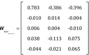
! ! ! w₁ displacement = 0.0005 0.005 0.008 '0.023 ⎡ ⎣ ⎢ ⎢ ⎢ ⎢ ⎤ ⎦ ⎥ ⎥ ⎥ ⎥ w₁

displacement₀ ='0.431

(3.25) ! ! ! w₂ displacement = 0.052 0.009 '0.324 '0.045 ⎡ ⎣ ⎢ ⎢ ⎢ ⎢ ⎤ ⎦ ⎥ ⎥ ⎥ ⎥ w₂

displacement₀ ='5.490

(3.26) ! ! ! w₃ displacement= 0.019 0.007 0.169 0.066 ⎡ ⎣ ⎢ ⎢ ⎢ ⎢ ⎤ ⎦ ⎥ ⎥ ⎥ ⎥ w₃

displacement₀ =)7.186

(3.27)

!

Σ_displacement=

3188.044 2203.698 386.171 311.242

2203.698 2678.795 281.599 332.173

386.171 281.599 100.443 72.613

311.242 332.173 72.613 96.763

(51)

[image:51.612.101.546.117.562.2]

Table 3.3: Confusion matrix for probabilistic generative classification using displacement data.

ALL DATA PREDICTED CLASSES

ACTUAL CLASSES Displacement Okay Over Under

Okay 97.4 1.4 1.2

Over 44 56 0

Under 38.4 0 61.6

Okay 95 1.4 3.6

Over 32 68 0

Under 17.6 0 82.4

Okay 97.8 1.4 0.8

Over 67.2 32.8 0

Under 63.2 0 36.8

AVERAGE

OF CROSS

VALIDATIONS

PREDICTED CLASSES

Okay 96.4 1.4 2.2

Over 49.6 50.4 0

Under 40.4 0 59.6

(52)

3.2 Discussion of Results for Tables 3.1 to 3.3

The confusion matrices show a consistent decrease in prediction performances

with decreasing frequencies (acceleration is dominated by high-frequencies, velocity by

mid-frequencies, and displacement by low-frequencies) although this decrease is not

significant. Cross validation using the first half of the data set for training and the rest for

validation produces reasonable prediction performances (at least more than 65 percent

accurate predictions). On the other hand, using the second half for training and the first

half for validation gives not so desirable cross validation results. This trend is seen in all

types of input: acceleration, velocity, and displacement. The simplest explanation is that

the models could be suffering from overfitting because we did not use a prior distribution

to provide regularization. We will propose a solution that is robust to overfitting by using

a full Bayesian treatment in the next sections.

3.3 Classification – Probabilistic Discriminative Model with Maximum Likelihood Estimate (MLE)

The following theory is based on the concepts described in Chapter 4, Linear

Models for Classification in Bishop, 2006.

In the previous section, we determined the parameters of the class-conditional

densities,

!

!p

( )

xCk , along with the class priors, _!p C

( )

k . Then, we used Bayes’ theorem to

compute the posterior class probabilities,

!

!p C

( )

k x . The posterior class probabilities are

given by a softmax function of a linear function of the input feature vector _!x. The

coefficients (parameters _!_!w_k and _!_!w_k0) of the linear function of !x are computed using the

parameters of the class-conditional densities, i.e., _!_!m_k and Σ and the class priors,

(53)

The advantage of the probabilistic generative model is that we can create (generate)

synthetic input values, _!x, by sampling from the marginal distribution

!

!p

( )

x . However,

the predictive performance may decrease, especially when the Gaussian form, which we

used to model the class-conditional densities, does not give a good representation. In this

section, we compute the parameter values in a more direct approach by maximization of

the likelihood function or the posterior probability density function (PDF). By not

modeling the class-conditional densities explicitly, we will have less number of

parameters to determine, and this may lead to an increase in predictive performance.

Directly determining the parameters is an example of a probabilisticdiscriminative

approach.

The likelihood function we want to maximize to determine the parameters

consists of the conditional distributions introduced earlier:

!

!p C

( )

k x . We start with a

relabeling of the variables first, and then we simplify as much as possible to avoid clutter

in our mathematical expressions. In the previous section, we obtained the functional form

of the posterior class probability, conditional on an input vector, as (3.4). Using this

definition, let us define

! ! !

y_k

( )

x =p C

(

_k x,w_k

)

= exp

(

ak

( )

x wk

)

exp

(

a_j

( )

x w _j

)

j

∑

(3.29)

where _!a_k are called activations and are given by

!

!ak

( )

x wk =wk

T_x_ _(3.30)

(54)

In the expression above,

!

!wk= wk0,wk T

(

)

T

and

! !

!x= 1,x

T

( )

T

, that is, we augment the input

vector with a dummy input _!_!x₀=1, similar to what we did in the least squares

classification in Appendix C. In order to decrease the clutter in the mathematical

notation, let us redefine the parameters (_!w →w and _!x→x) such that

!

!wk =

(

wk0,wk1,,wkD

)

T

and

! !

!x=

(

1,x1,x2,,xD

)

T

. Then, we consider maximization of

the likelihood function to determine the parameters

!

{ }

wk directly.

Now, we need the likelihood function. As we mentioned above, it consists of the

posterior class probabilities !

!p C

( )

k x if the prior on the !Ck’s is uniform. We will follow

the same _!_!1−of −K coding scheme as we did above for the target vectors: the target

vector _!_!t_n associated with the input vector _!_!x_n, which is assigned to class _!C_k, will be a

unit vector of dimension _!_!K=3 with each of its elements being zero unless it is the !kth

element, which is one. Then, we obtain the likelihood function as

! !

!p

(

T X,W

)

= p C

(

k xn,wk

)

t_nk

= y_nkt_nk

k=1 K

∏

n=1 N

∏

k=1 K

∏

n=1 N

∏

(3.31)

where the elements _!t_nk form the matrix _!T whose dimension is _!N×K with _!N as the

number of data points and _!K as the number of classes, and _!W is formed by _!_!D+1

-dimensional vector _!_!w_k as its _!kth_{column, and}

!X is formed by _!_!D+1-dimensional vector

!

!xn

T_{as its}

!nth row. So, _!W and _!X are matrices with dimensions

!

( )

D+1 ×K and

!

(55)

!

! !

y_nk= y_k

( )

x_n =p C

(

_k x_n,w_k

)

= exp wk T_x

n

(

)

exp w_jT_x

n

(

)

j

∑

∈⎡⎣ ⎤⎦0,1 (3.32)

Before we start evaluating the probabilistic discriminative model from a Bayesian

perspective, let us use the maximum likelihood method to find _!_!W_MLE by maximizing the

likelihood function given by (3.31). Note that the value we will find is in fact the

Bayesian maximum a posteriori (MAP) value but we are taking a flat (non-informative)

prior for _!W, so _!MAP≡MLE. I solved this optimization problem by an algorithm

provided by Matlab.

We maximized (3.31) with respect to _!W separately for acceleration, velocity, and

displacement input and obtained the following confusion matrices by assigning an input

vector !x to class _!C_k, where

!

!p C

(

k x,wk

)

is a maximum over !!k=1,2,3. Similar to the

previous confusion matrices, we show the predictive performance of our models by cross

validation; we divide the data sets into two: training data set and validation data set. Then

we swap these data sets and average the predictive performances in the form of confusion

matrices.

Let us start with acceleration results. The maximum likelihood estimate (MLE) of

the parameter matrix,

!

!WMLE_acceleration, computed using the entire acceleration data set for

(56)

! ! ! W MLE acceleration = 2.899 &0.003 0.002 &0.002 &0.008 &1.263 0.018 0.013 &0.118 &0.067 &1.606 0.003 &0.005 0.075 0.117 ⎡ ⎣ ⎢ ⎢ ⎢ ⎢ ⎢ ⎢ ⎤ ⎦ ⎥ ⎥ ⎥ ⎥ ⎥ ⎥ (3.33)

Table 3.4: Confusion matrix for probabilistic discriminative classification with MLE using acceleration data.