2017 2nd International Conference on Software, Multimedia and Communication Engineering (SMCE 2017) ISBN: 978-1-60595-458-5
A New Traffic Congestion Forecast Model Based on City Cell
Ruo-yu REN, Yong-jian YANG
*and Si-qi ZHAO
Computer Science and Technology, Jilin University, Jilin China
*Corresponding author
Keywords: City cell, Congestion forecast, Local-correlation.
Abstract. Solving the problem of urban traffic congestion has always been an important issue in urban development. By predicting the congested areas in the city, it can be dealt with more timely and alleviate traffic difficulties. This paper presents a traffic congestion prediction model based on local correlation of urban cells. Reducing the granularity of the analysis to the cell can effectively improve the efficiency of the area, and the local correlation takes into account the effect of regional and interregional traffic loading. The experimental results show that the accuracy and recall rate of the proposed model are good.
Introduction
Forecasting and dealing with traffic congestion in a timely manner in any country is a meaningful and worthy study. In the prediction of traffic congestion, many researchers take advantage of traffic data to make different research results. In [1], Kong Xiangjie et al. used the particle swarm optimization algorithm to predict the traffic flow parameters, and proposed a new traffic flow forecasting method. From the accuracy, instantaneity and stability of the three aspects of analysis, according to traffic flow distribution of the three weights. In [2], the authors predict the urban traffic flow through an integrated learning model with seven machine learning classification methods. In the paper[3], Y Ando et al. Have proposed a pheromone model, which takes the vehicle as the pheromone released by insects, and predicts the traffic congestion through the pheromone mechanism. In the[4], Pedro Lopez-Garcia, Enrique et al. proposed a genetic algorithm based on Onieva and cross entropy algorithm to predict traffic congestion. In [5], Han, Shi, Y, and others use random forest algorithm to predict real-time traffic congestion.
However, most of these methods are not only efficient when they are faced with complicated road conditions and huge data, but also with people for the emotional perception of congestion there are some differences. To sum up, the current congestion forecasting method still has some following problems:
1) The complexity of road-based analysis: the vast majority of the current model of the traffic patterns are based on road sections for the forecast, which need to record the city of each crossing gps data, Large cities have many large and or small sections, and each section of cross-vertical and horizontal, varying lengths, for some of the problems will cause difficulty.
2) Didn’t consider the influence of the overall urban space: some models only consider the temporal and spatial relationships of individual traffic areas, and they didn’t consider the impact of other areas on the traffic situation in the area.
a) b) c) d)
Figure 1. a) traffic segment analysis b) traffic city cell analysis c) city part congestion state d) city global congestion status.
Basic Definition and Preparatory Content
(Definition 1)Urban time-space trajectory: Within a time slot Tj. A collection of current gps points for a city (gps track point gi = {taxi_id, timestamp, latitude, longitude, Velocity, direction}).STC = {g1, g2, g3, ... gn | gi.timestamp Tj}
(Definition 2) City cell: a city cell refers to a city space-time track map, the urban space-time trajectory in the rectangle is divided into a number of length and width of a small rectangles, a small rectangle is a city cell. Each cell contains a collection of gps track points within a certain time slot and a range of cell geographic profiles.
(Definition 3) Urban cell density: Assume a city cell’s track point set is G = {g1, g2, g3, ..., gN},
N is the number of track points in the city cell, which represents the number of times to record in
this cell. We define the value of N as the density of the city cell like equation (1):
). |
( i
grid countgi gi gird
Density i (1) (Definition 4) Average cell speed in city: In a city cell, the gps trajectory point also contains attributes such as velocity. we define the city cell as the average speed of all the track points in the city cell. As shown in equation (2):
i i grid i i grid Density gird gi velocity g sum
Velocity ( . | )
. (2)
(Definition 5)Congestion value: Calculate the cell's congestion value with the speed and density attributes defined above. The city cell congestion value is defined as follows:
1 gird grid grid Velocity Density C (3)
Through the Definition 5, we can calculate the congestion value of a city cell. But the range of
value of city cells is too large, to this end, we do traffic discretization. After the discretization of the value of what we call the congestion state of the city cell.
As shown in Table 1: congestion state from 0-6 were divided into seven states, the greater the state value, indicating that the more congested areas.
Figure 1c and Figure 1d show the congestion state of the part city and the congestion state of the global city in a certain period of time, respectively.
[image:2.595.95.504.67.172.2]Table 1. The relationship between congestion value and congestion state.
Congestion value congestion state
=0 0
>0 and ≤2 1
>2 and ≤4 2
>4 and ≤6 3
>6 and ≤8 4
>8 and ≤10 5
>10 6
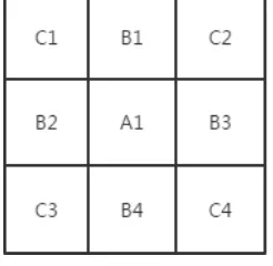
(Definition 7) Geo-related_City cells: In a city, city cells that present adjacent relationships (with one side in common) are geographically related to each other.
As shown in Figure 4a), the region A1 is the target region, and the regions B1, B2, B3, B4 are the Geo-related_City cells of the region A1. Although the regions C1, C2, C3, and C4 are located at the four corners of the target region A1, they do not belong to the Geo-related_City cells of A1.
Figure 2. Geo-related city cells.
Local Correlation Model
In the local correlation model, the main consideration is the target city cell and its adjacent city cell vehicle flow into and out. If four neighboring city cells enter the target city cell traffic flow more than the target cell out of traffic flow, and the average speed slows down, this will cause the target city cell more jammed than the previous time period, otherwise it will change smooth. City cells are bounded by edges, a city cell has four sides, and there are four directions of traffic. Each direction has a certain number of traffic and average flow rate. It can also be said that in the same city cell, the four directions have their own congestion situation.
(Definition 9) Escape flow: The flow enters the adjacent cell from the target cell, and plays a role in the traffic state of the target city cell, as shown in Figure 3.
(Definition 10) Driving Flow: The traffic enters the target cell from the adjacent cell, and the traffic state of the target city cell is congested, as shown in Figure 3.
(Definition 11) Traction flow: Here, there are two traction forces affecting the grid congestion state, as shown in Figure 3, F3 and F4. Are respectively the escape forces of the adjacent cells and the target cell at the other end of the adjacent side.
Figure 3. Three types flow of local correlation cells.
For the target city cell, it has four sides, for each edge E, the target cell flow from E to the adjacent cell, forming an escape force (Figure 3 F1), the adjacent cell from the edge E Into the target cell, the formation of driving force (Figure 3 F2). At the same time, there are two traction (Figure3 F3, F4) affect the escape force and driving force. For the escape force, if the F3 on behalf of the traffic faster and smoother to accelerate the F1 flee, help to alleviate the target cell congestion, if the F3 on behalf of the traffic flow more slowly and more congestion will slow down the escape of F1, is not conducive to Target cell flow. Similarly, the role of F4 on the driving force is also true. Therefore, the impact of an adjacent cell on the target cell can be represented by these four forces.
As shown in Figure 3, the influence of urban cell B1 on the congestion of the target city cell by edge E1 is shown in the following formula:
4 2 2 3 1 1
1 F
e F e
CB A F F F F
(4) Each force is determined by the number of traffic flows along the direction of the force in a certain time slot, the average vehicle speed of the vehicle, and the specific congestion of the grid. α and β are constants, represents the influence of some other factors.
The destination cell has four adjacent cells. Suppose the current time slot is T, the next time slot T + 1, the congestion value of cell A is:
A B A B A B A B
A C C C C
C 1 2 3 4 . (5)
Experiment and Results
Evaluation Criteria
We use the accuracy and recall as the evaluation criteria, accuracy is defined as the proportion of all predicted results obtained by the training set to be obtained from the model output on the test set, i.e.:
N T true
accurcy ( ) . (6)
Where True (T) represents the number of cities in the T time slot prediction results consistent with the actual situation, N represents the total number of test centralized city to predict the cell.
The recall rate is defined as follows:
M count(M)
4
f(i)
i
recall
(7) The M is the set of cells in the city where the traffic state is congested in next time slot, and the
Experiment Procedure
The experiment selected the Beijing taxi’s gps trajectory data set in April 2012, the day of the time piece by every half hour division, a total 48 of time slots, and 48 time slots by 1-48 sort. The significance of the local correlation congestion prediction model is to predict the congestion status of the next time slot of the target cell by the current time slot target cell and the congestion state of its neighboring cells, wherein the first time slot state of the next time slot is predicted with the 48th time slot.
Each time slot is predicted according to the local correlation model, and its corresponding accuracy rate and recall rate are shown in Figure 4:
a) b)
Figure 4. a). The accuracy of each time slot, b) the recall of each time slot.
As can be seen from the Figure 4, the accuracy in the early morning and night is relatively high,
but in the daytime, especially in the morning and evening peak period there will be a certain decline, because in the early morning or at night when the vehicle is relatively less, The traffic is also stable, there are no other complex factors, and most areas without vehicle driving or very few vehicles driving. But in the daytime, especially in the morning and evening peak, congestion is more complex, each cell is different from the situation of each cell, there are many reasons for congestion, no longer only adjacent areas of the factors. Therefore, the accuracy rate will be reduced. In addition, the recall rate fluctuates greatly in the early morning and night, while during the daytime it is kept at a relatively stable value. This is because the early morning and night congestion is not much, the base is small and the speed is relatively fast; each area of the congestion changes will quickly. However, during the daytime, there are many congested areas, and the congestion problem in the area is not solved for a short time, so the recall rate is maintained within a stable range.
Concluding Remarks
It can be seen from the experiment that the model proposed in this paper has certain effect in predicting traffic congestion, and the calculation complexity is low and also has certain stability, which suggests that the interaction between regions in urban traffic is more pronounced. However, when the current urban environment becomes complex, the predictive effect of the model will decline. So in our future work, we combine the city's temporal and spatial environment, they will cause congestion factors to consider more comprehensive. In this paper the status of each city cell is the same, but in real life the different areas of the city because of its geographical location and the ownership of the building has a different role and weight, which our work needs further consideration.
References
[image:5.595.74.523.214.383.2]floating car trajectory data[J]. Future Generation Computer Systems, 2016, 61:97-107.
[2] Asencio-Cort, S, G, Florido E, et al. A novel methodology to predict urban traffic congestion with ensemble learning[J]. Soft Computing - A Fusion of Foundations, Methodologies and Applications, 2016, 20(11):4205-4216.
[3] Ando Y, Masutani O, Sasaki H, et al. Pheromone model: application to traffic congestion prediction[C]// International Joint Conference on Autonomous Agents and Multiagent Systems. DBLP, 2005:1171-1172.
[4] Lopez-Garcia P, Onieva E, Osaba E, et al. Hybridizing Genetic Algorithm with Cross Entropy for Solving Continuous Functions[C]// Genetic and Evolutionary Computation Conference. 2015:763-764.