R E S E A R C H
Open Access
On bounds for solutions of monotonic first order
difference-differential systems
Javier Segura
Correspondence: javier. segura@unican.es
Departamento de Matemáticas, Estadística y Computación. Facultad de Ciencias. Universidad de Cantabria, 39005-Santander, Spain
Abstract
Many special functions are solutions of first order linear systems
yn(x) =an(x)yn(x) +dn(x)yn−1(x),yn−1(x), =bn(x)yn−1(x) +en(x)yn(x). We obtain bounds for the ratiosyn(x)/yn-1(x) and the logarithmic derivatives ofyn(x) for solutions
of monotonic systems satisfying certain initial conditions. For the casedn(x)en(x) > 0,
sequences of upper and lower bounds can be obtained by iterating the recurrence relation; for minimal solutions of the recurrence these are convergent sequences. The bounds are related to the Liouville-Green approximation for the associated second order ODEs as well as to the asymptotic behavior of the associated three-term recurrence relation asn®+∞; the bounds are sharp both as a function ofnandx. Many special functions are amenable to this analysis, and we give several examples of application: modified Bessel functions, parabolic cylinder functions, Legendre functions of imaginary variable and Laguerre functions. New Turán-type inequalities are established from the function ratio bounds. Bounds for monotonic systems with dn(x)en(x) < 0 are also given, in particular for Hermite and Laguerre polynomials of
real positive variable; in that case the bounds can be used for bounding the monotonic region (and then the extreme zeros).
Mathematics Subject Classification 2000: 33CXX; 26D20; 34C11; 34C10; 39A06.
Keywords:monotonic difference-differential systems, Riccati equation, three-term recurrence relation, special function bounds, Tur?á?n-type inequalities, zeros of ortho-gonal polynomials
1 Introduction
Many special functions, and in particular functions of hypergeometric type, satisfy first order differential systems of the form
yn(x) =an(x)yn(x) +dn(x)yn−1(x),
yn−1(x) =bn(x)yn−1(x) +en(x)yn(x).
(1)
For the particular case of modified Bessel functions sharp bounds for function ratios yn(x)/yn-1(x) and logarithmic derivatives yn(x)/yn(x), as well as Turán-type inequalities were recently obtained in [1]; the key ingredient in the analysis was the study of the qualitative behavior of the solutions of the Riccati equation satisfied byhn(x) = yn(x)/ yn-1(x), together with the application of the three-term recurrence relation.
In this article, the ideas in [1] are generalized and applied to a much broader set of functions. We analyze the qualitative behavior of the Riccati equation associated to the ratiohn(x) = yn(x)/yn-1(x),
hn(x) =dn(x)−(bn(x)−an(x))hn(x)−en(x)hn(x)2, (2) in the general case in which the quadratic equation
en(x)λn(x)2+ (bn(x)−an(x))λn(x)−dn(x) = 0 (3) has two distinct real roots λ±n(x). This case corresponds to monotonic systems, with solutions which have one zero at most. As we will see, if the functions λ±n(x) are monotonic, they are bounds for the ratios hn(x) satisfying certain initial value
conditions.
The methods can be applied to many special functions, modified Bessel functions, parabolic cylinder functions, Legendre and Laguerre functions among them. Ratios of Bessel functions appear in a great number of applications, particularly as parameters of certain probability distributions (see, for instance, the examples mentioned in [1]). Parabolic cylinder ratios appear in the study of Ornstein-Uhlenbeck processes (see, for instance [2]), and other special function ratios (Whittaker, Legendre, Gauss hypergeo-metric functions) play similar roles as well [3-5]. In all these applications, a common characteristic is that the functions are real and the variables lie inside a monotonic region (region free of zeros). These are precisely the conditions under which our tech-niques can be applied.
In addition to direct applications in several areas, particularly in statistics and stochas-tic processes, the bounds on function ratios have implications in the construction of numerical algorithms. These techniques provide bounds for the region of computable parameters of a given function within the overflow and underflow limitations, and they also provide bounds for the condition numbers of the functions (see Section 4.1.2 for the case of parabolic cylinder functions). Additionally, as discussed for the particular case of modified Bessel functions [1], the bounds are useful for accelerating the conver-gence of certain continued fraction representations which are used in numerical algo-rithms; for instance, the algorithms in [6,7] could be improved by using the bounds of Sections 4.1.2 and 4.1.3 for accelerating the convergence.
We obtain upper and lower bounds for function ratios and logarithmic derivatives of the solutions of systems (1) withdn(x)en(x) > 0. The bounds are accurate for large values
of the variablexand the parametern. This is a consequence of the connection between the bounds, the Liouville-Green approximation for the associated second order ODE and the asymptotic behavior of the associated three-term recurrence relation. We also give two examples of applications of the methods for the case dn(x)en(x) < 0 (Section
4.2) and use these results for bounding function ratios for Laguerre and Hermite polyno-mials in the real axis (but outside the oscillatory region). These bounds can be used for bounding the oscillatory region and, therefore, for bounding the extreme zeros.
The structure of the paper is as follows. In Section 2 we analyze the conditions which guarantee that the roots of (3) are bounds for the ratiosyn(x)/yn-1(x). The dependence
onnis analyzed in Section 3. The use of the three-term recurrence relation allows us to obtain sequences of upper and lower bounds in the case dn(x)en(x) > 0; Turán-type
2 Qualitative behavior of riccati equations
We consider first order differential systems (1) with differentiable coefficients, for which the ratiohn(x) =yn(x)/yn-1(x) satisfies the Riccati equation
h(x) =d(x)−(b(x)−a(x))h(x)−e(x)h(x)2. (4) The label n, which is common for h and the coefficients a, b, d and e, has been dropped in (4) for simplicity. The analysis in this section is valid for any system, depending or not on a parametern. The explicit dependence onnwill be recovered in the next section.
We haveh’(x) = 0 whenh(x) =l±(x) with
λ±(x) = sign(e(x))R(x)−η(x)±η(x)2 +s
,
R(x) =
de((xx)),η(x) = b(x)−a(x) 2d(x)e(x)
,s= sign(d(x)e(x)),
(5)
We consider the case with real roots l±(x). Two distinct situations may occur: either d(x)e(x) > 0, ord(x)e(x) < 0 but |h(x)| > 1.
The conditiond(x)e(x) > 0 generally holds in the whole maximal interval of continu-ity of the functions because the coefficients d(x) and e(x) do not change sign under very general conditions (see, for instance, [[8], Lemma 2.1]). Contrarily, when d(x)e(x) < 0 the condition |h(x)| > 1 may hold only for a limited range of the variablex. In the first case (d(x)e(x) > 0)h(x) may have one zero or one singularity, but not both ([[8], lemma 2.4]), while in the secondh(x) may have both a zero and a singularity [[9], The-orem 2.1]. We analyze the case d(x)e(x) > 0, assuming that no change of sign ofh(x) occurs. For the case d(x)e(x) < 0, as the examples in Section 4.2 will show, similar arguments can be applied.
In the sequel, we considerd(x)e(x) > 0. Without loss of generality, we taked(x) > 0,e (x) > 0 and thenl+(x) > 0 andl-(x) < 0; ifd(x) < 0,e(x) < 0 we can consider the repla-cement y®-yor w®-w. In the next results, (a, b) is an interval whereh(x) and the coefficients of the system are differentiable;aorb could be +∞or -∞. Depending on the value of h(x) ata+or b-different bounds can be established. First we considerh(a +
) > 0. We enunciate three results and give a common proof.
Lemma 1.If h(a+) > 0then h(x) > 0in(a, b)
Theorem 1.If h(a+) > 0,l+(x)is monotonic and h’(a+)l+’(a+) > 0then(h(x) -l+(x))l +’
(x) < 0in(a, b).
Theorem 2. If h(a+) > 0, l+(x)is monotonic and h’(a+)l+’(a+) < 0then either h(x) reaches one relative extremum at xeÎ(a, b) (a minimum if l+’(x) > 0and a maximum ifl+’(x) < 0)or(h(x) -l+(x)) l+’(x) > 0in(a, b).
Proof. Ifh(a+) > 0, then h(x) can not change sign continuously: it can not become zero because h’(x) > 0 if 0≤ h(x) < l+(x). On the other hand, it can not change sign discontinuously; for this, starting withh(a+) > 0, a valuex∞Î (a, b) should exist such that h(x−∞) = +∞ but this is not possible becauseh’(x) < 0 ifh(x) >l+(x).
Assume first thath’(a+) > 0; using (4) this means that 0 <h(a+) <l+(a+). And then, necessarily h(x) <l+(x) in (a, b). Indeed, becausel+(x) is monotonically increasing and the graph of h(x) is below the graph of l+(x) close to x = a, the graph ofh(x) may touch the graph ofl+(x) atx = xeonly if the first one has a larger slope at xe, that is,
ifh’(xe) >l+’(xe) > 0; but ifh(xe) =l+(xe) thenh’(xe) = 0.
Assume now thath’(a+) < 0. The graph ofh(x) lies above the graph of l+(x) close to x = a and there are two possibilities: either it remains abovel+(x) in all the interval or there is a point xe Î (a, b) where h(xe) = l+(xe) andh’(xe) = 0. The graph of h(x)
crosses the graph of l+(x), which is an increasing function, andh’(x) > 0 for allx>xe.
Therefore there is a minimum at xe.
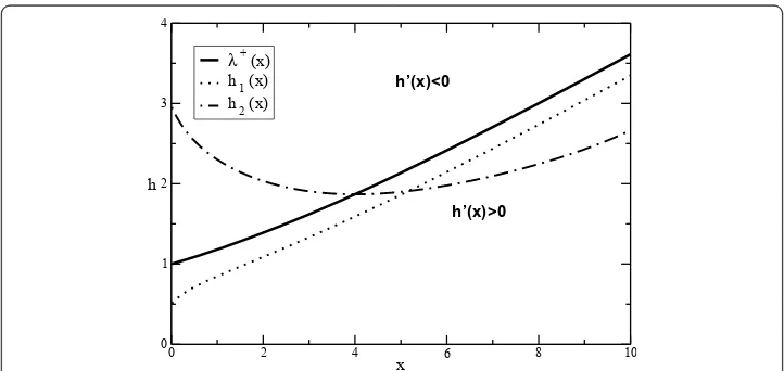
Figure 1 illustrates the situations described in Theorems 1 and 2.
If, differently from Theorems 1 and 2, we have h(a+) < 0 thenh(x) may change sign once. But if it does not change sign and h(b-) < 0 we are in the previous situation. Indeed, with the change of variable x® -xand the change of functionw(x)® -w(x),
we have that the new ratio of functions h˜(x) =−y(−x)/w(−x) is such thath˜(α+)>0
and the previous results hold in the interval [a, b] = [-b, -a]. Then, we can write a common result for both cases. We only give the result corresponding to Theorem 1.
Theorem 3.Let h(x)be a solution of (4)with continuous coefficients and d(x) > 0,e (x) > 0.Suppose that either h(a+) > 0or that h(b-) < 0 and take s = +, c = a+in the first case and s = -, c = b-in the second. Then, h(x)does not change sign in(a, b),and if the characteristic root ls(x)is monotonic andls’(c)h’(c) > 0then
h(x)−λs(x)dλ
s
dx <0 ∀x∈(a,b)
Remark 1.The conditionls’(c)h’(c) > 0is equivalent to
h(c)−λs(c)dλ
s
dx(c)<0
0 2 4 6 8 10 x
0 1 2 3 4
h
λ + (x) h 1 (x) h 2 (x)
[image:4.595.117.478.524.695.2]h’(x)>0 h’(x)<0
Figure 1The characteristic rootl+(x) divides the plane in two regions:h’(x) > 0 if 0 <h(x) <l+(x) andh’(x) < 0 ifh(x) >l+(x). The graph ofh1(x) corresponds to the situation described in Theorem 1
3 Bounds for first order DDEs
Now, consider a first order difference-differential equation (1) and assume it holds for n≥ n0and that it is possible to make the shift n®n +1 in (1). In this case the
solu-tions of (1) are also solusolu-tions of a three-term recurrence relation
en+1yn+1(x) + (bn+1(x)−an(x))yn(x)−dnyn−1(x) = 0. (6)
As in the previous section, we assume dn(x)en(x) > 0.
Let λ¯±n be the roots of the algebraic equation
en+1λ¯2n+ (bn+1−an)λn¯ −dn= 0, (7)
that is
¯
λ±
n =RnEn − ¯ηn±
1 +η¯2
n
,
Rn=dn/en,En=en/en+1, ηn¯ = (bn+1−an)/
2dnen+1
(8)
If limn→+∞ηn¯ = 0 then limn→+∞¯λ+n/λ¯−n= 1, and if the coefficients are of algebraic
growth as a function of n, Perron-Kreuser theorem (see [[10], Theorem 4.5]) states
that independent pairs of solutions y(1)k ,y(2)k exist such that
lim
n→+∞ 1 ¯
λ+
n y(1)n
y(1)n−1 = 1, limn→+∞ 1 ¯
λ−
n y(2)n
y(2)n−1 = 1. (9)
If ηn¯ >0 the minimal solution is yn(1) and yn(2) is dominant, and therefore
limn→+∞y(1)n /y(2)n = 0 Ifhn< 0 the roles are reversed. In both cases we have, for
suffi-ciently large n, yn(1)+1yn(1)>0 and y(2)n+1y (2)
n <0.
Remark 2.The minimal solution satisfies ηnyn¯ /yn−1>0 for large n, while the domi-nant solutions are such that ηn¯ yn/yn−1<0 for large n.
Notice that the roots (8) are closely related to the characteristic roots of the Riccati equation (5):
λ±
n(x) =
dn(x)
en(x) −ηn(x)±
1 +ηn(x)2
,ηn(x) = bn(x)−an(x)
2dn(x)en(x). (10)
As we have shown in the previous section, when λ±n(x) are monotonic they provide bounds for some solutions. On the other hand, if limn→+∞λ¯±n/λ±n = 1 the function
ratios have these bounds as limits. This explains why the bounds (10) tend to be shar-per as nbecomes larger. Because of this, we refer to these bounds as Perron-Kreuser bounds.
In Section 3.2 we will obtain additional upper and lower sharp bounds starting from the bounds of Theorem 1 and using the three-term recurrence.
3.1 Monotonicity of the characteristic roots
The next result relates the monotonicity properties of the characteristic roots with the monotonicity properties as a function ofn.
Theorem 4. Let yk(x), k = n, n - 1, be solutions of second order ODEs
yk(x) +Bk(x)yk(x) +Ak(x)yk(x) = 0, with Ak(x),Bk(x)continuous in(a, b)and Bn(x) = Bn-1(x).Assume that yn(x)and yn-1(x)satisfy a system(1)with dn(x)en(x) > 0and differ-entiable coefficients. Then, en(x)/dn(x)is constant as a function of x, and if An(x)≠An-1
(x)the characteristic roots λ±n(x) (10)are monotonic in (a, b).Furthermore, dλ±n(x)/dx
has the same sign as An-1(x) -An(x)and −ηn(x).
Proof. Differentiating the first equation of the system (1) and eliminating yn-1 and
proceeding similarly with the second equation we have
yk(x) +Bk(x)yk(x) +Ak(x)yk(x) = 0, k=n, n−1, (11) with coefficients satisfying:
Bn(x)−Bn−1(x) = e
n(x) en(x)−
dn(x)
dn(x),
An(x)−An−1(x) =bn(x)−an(x)−bn(x)e
n(x) en(x)+an(x)
dn(x)
dn(x)
(12)
Now, because we are assuming that Bn(x) =Bn-1(x) the first equation implies that dn
(x)/en(x) does not depend on x. Therefore, from the expression of the characteristic
roots (8) we see that dλ±n(x)/dx has the same sign as −ηn(x). All that remains to be proved is that An(x) - An-1(x) has the same sign as ηn(x). But considering the second equation of (12) and using that dn(x)/dn(x) =en(x)/en(x) one readily sees that
An(x)−An−1(x) = 2dn(x)en(x)ηn(x), which proves the theorem.
Remark 3.If en(x)dn(x) < 0andhn(x)2 > 1,it is also true that both roots are
mono-tonic if Bn(x) = Bn-1(x)and An(x)≠An-1(x),but λ+n(x)λ−n(x)>0 and λn+(x)λ−n (x)<0
in this case.
The case described in Theorem 4 is, for instance, the situation for Bessel functions, parabolic cylinder functions and the classical orthogonal polynomials when nis the degree of the polynomials.
3.2 Perron-kreuser bounds
In the following, we assume that hn(x), ηn¯ (x),dn(x),en(x) andhn(x) = yn(x)/yn-1(x) do
not change sign for large enough n(sayn≥n0). Notice that the sign condition for hn
(x) is satisfied for large enough nwhen Perron-Kreuser theorem holds. An immediate application of Theorem 3 gives:
Theorem 5 (First Perron-Kreuser bound).Let dn(x) > 0,en(x) > 0and hn(x) = yn(x)/ yn-1(x) with constant sign for n ≥ n0 and for any x Î (a, b). Let s = sign(hn(x)) and
λs
n(x) as in Equation (10).Then, if hn(a+) > 0 andhn(a+)λs
n(a+)>0or hn(b-) > 0 and
hn(b−)λs
n(b−)>0 the following holds in(a, b):
hn(x)−Fns(x)
λs
Fsn(x) =Rn(x) −sηn(x) +
1 +ηn(x)2
= Rn(x)
sηn(x) +
1 +ηn(x)2 (14)
Further bounds can be obtained by iteration of (6), which we write:
yn(x)
yn−1(x)=dn bn+1−an+en+1
yn+1(x)
yn(x) −1
. (15)
For minimal solutions we have that ηn¯ (x)yn(x)/yn−1(x)>0 for largen. By
substitut-ing in the previous equation yn+1(x)/yn(x) by a lower (upper) bound we get an upper
(lower) bound for yn(x)/yn-1(x). The process can be iterated to produce sequences of
lower and upper bounds. We only give the first iteration.
Theorem 6(Second Perron-Kreuser bound for minimal solutions). Under the
condi-tions of Theorem5and if sηn¯ >0,s=sign(hn)then
hn(x)−Ssn+λns(x)>0, n≥n0 (16)
where
Ssn+= DnEnRn
s(2Dnηn¯ −ηn+1) +
1 +η2
n+1
(17)
Dn=dn/dn+1 En, Rnand ηn¯ given by(8)andhnby(10).
The second superscript of the notation Ss+
n stands for the sign of ηnyn¯ /yn−1.
Notice that Theorem 6 may be true for n = n0- 1 too, because Theorem 5 is used in
the proof with the shiftn®n+ 1.
The similarity of the second expression of (14) with (17) indicates that for coeffi-cients of algebraic growth we will generally have limn→+∞Fns/Ssn+= 1.
Further iterations are possible and this gives a convergent sequence of upper and lower bounds under the conditions of Theorems 5 and 6 and provided that Perron-Kreuser theorem holds (which implies that the recurrence admits a minimal solutions). We don’t prove this result, but the convergence of the sequence of bounds for the minimal solution follows immediately by using the same arguments considered in [1] for the case of Modified Bessel functions of the first kind.
We can also obtain additional bounds for dominant solutions by writing
yn(z)
yn−1(x)
=−bn−an−1
en
+ dn−1
en
yn−2(z)
yn−1(z)
(18)
Differently from the case of minimal solutions, the sequence of bounds is not a con-vergent sequence. We give an explicit formula for the first iteration:
Theorem 7 (Second Perron-Kreuser bound for dominant solutions).Under the
con-ditions of Theorem5and if sηn¯ −1<0,s=sign(hn),
hn(x)−Ssn−λns(x)>0, n≥n0+ 1 (19)
where
Ssn−=Dn−1En−1Rn −s(2E−n−11ηn¯ −1−ηn−1) +
1 +η2n−1
Notice that the previous theorem can only be guaranteed to be true forn = n0 + 1,
because Theorem 5 is used in the proof with the shift n® n- 1.
The similarity of the first expression in (14) with (20) is clear. For coefficients of algebraic growth we will generally have limn®+∞ limn→+∞Fns/Ssn−= 1.
3.3 Turán-type inequalities
Turán-type properties for special functions have received a considerable attention in recent years; just to cite five different groups of researchers, we mention [1,11-14] (see also references cited therein). Turán-type inequalities can be obtained from the bounds on function ratios.
Indeed, because upper and lower bounds are available for |yn/yn-1| both whenynis a
minimal or a dominant solution (Theorems 5, 6 and 7), upper and lower bounds for |yn/yn-1||yn/yn+1| become available. The modulus can be skipped if yn/yn-1does not
change sign (as assumed earlier). With this:
ln≤Ln(x)< yn(x)
yn+1(x)
yn(x)
yn−1(x) <
Un(x)≤un, (21)
where ln=minx{Ln(x)} andun= maxx{Un(x)}. Many new Turán-type inequalities are
found in Section 4 by using this simple idea.
3.4 Bounds of liouville-green type
Using the difference-differential system (1) and the Perron-Kreuser bounds, bounds on the logarithmic derivatives can be established. We give the bounds obtained from the first Perron-Kreuser bound.
Theorem 8.Under the hypothesis of Theorem5 and if dλs
n/dx>0(s = sign(yn(x)/yn-1
(x))):
sy
n−1(x)
yn−1(x)<s
an(x) +bn(x)
2 +
dn(x)en(x)
1 +ηn(x)2<sy
n(x)
yn(x) (22)
If dλsn/dx<0 the inequalities are reversed
Two consequences follow. First, we observe that the ratios yk(x)/yk(x) are mono-tonic as a function of the discrete variable k. Second, because we are assuming that the shift n ® n + 1 is possible, we have both an upper and a lower bound for yn/yn. Upper and lower bounds could also be obtained by considering both the first and sec-ond Perron-Kreuser bounds.
In the examples we will see that these bounds, after integrating the logarithmic deri-vative, are related to the Liouville-Green approximation for solutions of second order ODEs. In fact, using this analysis and by Liouville-transforming the first order system associated to the ODE y″(x) +A(x)y(x) = 0, conditions can be established under which the LG approximation for the solutions of the ODE y″(x) +A(x)y(x) = 0 are bounds for some of the solutions. We leave this analysis for a future article.
4 Applications
We give a number of examples of application of the techniques described in the article. We focus on the case dn(x)en(x) > 0, but examples of application for monotonic
0",1,0,1,0,0pc,0pc,0pc,0pc>4.1 Cases withdn(x)en(x) > 0
We analyze three families of functions, which have as particular cases some classical orthogonal polynomials outside the interval of orthogonality In all cases Theorem 4 holds, with the exception of Laguerre functions of negative argument. In this case The-orem 4 can not be applied but the characteristic roots are still monotonic and the same analysis is therefore possible. Some monotonicity properties for the determinants of some of the functions analyzed were considered in [15].
4.1.1 Modified bessel functions
These are solutions ofx2y″+xy’-(x2+ν2)y= 0. This was the case considered in detail in [1], and most of the results obtained in that paper are direct consequences of the more general results of the present one.
4.1.2 Parabolic cylinder functions
The parabolic cylinder functionU(n, x) is a solution of the differential equationy″(x) -(x2/4+ n)y(x) = 0, with coefficientA(x) = - (x2/4+ n) depending monotonically on the parametern(Theorem 4 holds).
Considering the DDE satisfied by U(n, x) [[16], 12.8.2-3] and defining yn(x) =eiπnU
(n, x) we have:
yn(x) = x
2yn(x) +yn−1(x),
yn−1(x) =−x
2yn−1(x) + (n−1/2)yn(x).
(23)
wherenwill be real and positive. For this system
ηn(x) =− x
2n−1/2,ηn¯ (x) =ηn+1(x),λ ±
n(x) =
−2
x∓√4n−2 +x2 (24)
From [[16], 12.9.1] we have hn(+∞) = 0-and hn(+∞) = 0+ and because λ−n(+∞) = 0+ then Theorem 3 holds, as well as Theorems 5 and 6. Therefore
Theorem 9.For n> 1/2and x≥0the following holds
2
x+√4n+ 2 +x2 <
U(n,x)
U(n−1,x) <
2
x+√4n−2 +x2 (25)
The lower bound also holds if nÎ (-1/2,1/2)and it turns to an equality if n = -1/2. The lower bound is obtained from the upper bound and the application of the three-term recurrence relation: ifBm(n, x) is a positive upper (lower) bound for U(n, x)/U(
n-1,x),x> 0, then
Bm+1(n,x) = 1/(x+ (n+ 1/2)Bm(n+ 1,x)) (26) is a lower (upper) bound for the same ratio. The process can be continued asm®+∞ and the sequence is convergent (becauseU(n, x) is minimal).
Now, consider yn(x) = U(n, -x), which is also solution of (23). Using the values of U
Theorem 10.For n> 3/2and x≥0the following holds
x+√4n−6 +x2 2n−1 <
U(n,−x)
U(n−1,−x) <
x+√4n−2 +x2
2n−1 (27)
The upper bound is also valid if n Î(1/2, 3/2).
The upper bound in (25) has the same expression as (27) but with xreplaced by -x. Therefore:
Remark 4. Theorems9 and10 hold for all real x, but for x< 0the lower bound of Theorem 9 only holds for all x< 0 if n > 1/2. The lower bounds are sharper when x s> 0.
The following Turán-type inequalities are obtained from Theorems 9 and 10:
Theorem 11.Let F(x) =U(n, x)2/(U(n -1,x)U(n+ 1,x)).Then, for all real x:
n−3/2
n+ 1/2 <
n−1/2
n+ 1/2F(x)<1<F(x)<
n+ 3/2
n−1/2 (28)
The first inequality holds for n > 3/2 and the rest for n > 1/2. For x < 0the third inequality also holds if nÎ(-1/2, 1/2).
Finally, considering Theorem 8 and writing together the results forU(n, x) andU(n, -x) we have the next result.
Theorem 12.For all real x and n≥1/2the following holds:
−x2/4 +n+ 1/2< U(n,x)
U(n,x) <−
x2/4 +n−1/2 (29)
The left inequality also holds for n> -1/2.
These type of bounds are useful for studying the attainable accuracy of methods for computing the functions. In [17], the following estimation for large xand/ornwas
considered for the condition number with respect tox:
Cx(U(a,x)) =xU(a,x)/U(a,x)∼x
x2/4 +a, (30)
and similarly forV(a, x). The bounds (29) prove that this a good estimation because it lies between the upper and lower bounds. From the previous discussion on theV(a, x) function, one can prove that similar bounds are valid for moderatex(x> 1 is enough); we consider later this function.
Integrating (29) we have
Fn+1/2(x)/Fn+1/2(y)< U(n,y)
U(n,x)<Fn−1/2(x)/Fn−1/2(y),
Fα(x) = exp x 2
x2/4 +α
x+ 2
x2/4 +α
α (31)
and, in particular,
Fn+1/2(x)< U(a,x)
where
Fα(x) = exp ⎛ ⎝−x
2
x2 4 +α
⎞ ⎠
⎛
⎝ x
2√α +
x2 4α + 1
⎞ ⎠
−α
(33)
The bounds (32) are useful for obtaining the range of parameters for which function values are computable within the arithmetic capabilities of a computer (overflow and underflow limits). These results confirms the estimations based on the Liouville-Green approximation used in [18].
° Iterated coerror functions and Mill’s ratio:In particular, considering Theorem 9 and the relation of parabolic cylinder functions U(n+ 1/2,x) with the iterated coerror functionsinerfc(x) [[16], 12.7.7],nÎN, the following follows:
Mn+1(x)< i
nerfc(x)
in−1erfc(x)<Mn(x), n= 1, 2,. . .;Mn(x) =
x+√2n+x2−1. (34)
These inequalities appear in [19].
Theorem 9 also gives bounds on Mill’s ratio (n = 1/2). From the lower bound in Theorem (9) and the upper bound obtained by iterating with (26) we have
Theorem 13.Let r(x) =ex2/2+∞
x e−t
2/2
dt,then 2
x+√x2+ 4 <r(x)< 4
3x+√x2+ 8 (35)
The lower bound was obtained in [20] and the upper bound in [21]. In our case, these results follow from a more general result. See also [22] for an alternative proof.
Further iterations (see (26)) give additional sharper bounds:
Theorem 14.
R2k+1<r(x)<R2k(x) (36)
Rn(x) = 1
x+ 1
x+ 2
x+. . .
n Tn(x),Tn=
x+√4n+x2/2 (37)
where, as usual we denote 1 a+
1
b+· · ·= 1/(a+ 1/(b+· · ·))
°Hermite polynomials of imaginary variable: A similar analysis to that forU(n, -x) can be carried for the PCF V(n, x). Indeed, yn(x) = V(n, x)/Γ(n+ 1/2) is a solution of
(23) and hn(x) =yn(x)/yn-1(x) is such thathn(0+) > 0. Two situations take place
depend-ing on the values of n. First, ifn Î (2k -1, 2k), k Î N, then hn(0+)>0 the upper
bound of Theorem 10 holds for all x> 0 while the lower bound will hold fornÎ(2k, 2k + 1). Contrarily, ifn Î (2k, 2k + 1) then hn(0+)<0, while hn(+∞) > 0, and the
upper bound only holds for large enough x;a similar situation occurs with the lower bound whennÎ(2k -1, 2k).
Theorem 15.
V(n,x)
V(n−1,x) <
x+√4n−2 +x2
2 , x>0, n∈(2k−1, 2k), k∈N (38)
x+√4n−6 +x2
2 <
V(n,x)
V(n−1,x), x>0, n∈(2k, 2k+ 1), k∈N (39)
−iH2k+1(ix) H2k(ix) <
x+√4k+ 2 +x2 x>0, k= 0, 1, 2. . . (40)
iH2k−1(ix) H2k(ix) <
x+4k−2 +x2 −1
, x>0, k∈N (41)
H2k(ix)2 H2k−1(ix)H2k+1(ix) >
k−1/2
k+ 1/2, k∈N, x∈R. (42)
Hermite polynomials of imaginary argument were also considered in [15]. The well-known Turàn-type inequality for Hermite polynomials [23]Hn(x)2 -Hn-1(x)Hn+1(x) > 0, x Î ℝ, does not hold on the imaginary axis, but a similar property
Hn(ix)2−(n−1)/(n+ 1)Hn
−1(ix)Hn+1(ix)>0 holds true for allx> 0 ifnis even.
4.1.3 Oblate legendre functions
These are Legendre functions of imaginary argument, which are functions appearing in the solution of Dirichlet problems in oblate spheroidal coordinates [6]. Denoting
pn(x) =e−inπ/2Pmn(ix) (43)
and using the differential relations [[16], 14.10.4-5] we have
pn(x) = 1
1 +x2{nxpν(x) + (n+m)pν−1(x)}
pn−1(x) = 1
1 +x2{−nxpν−1(x) + (n−m)pν(x)}
(44)
and qn(x) =Qm
n(ix), Qmn being the second kind Legendre function, satisfies the same system. We consider n > m and x > 0. This is again an example for which Theorem 4 holds. The roles played in this case by the functions Qm
n(ix) andPmn(ix) are very simi-lar to the roles of U(n, x) and V(n, x) in the previous section. We omit details and only summarize the main results.
Theorem 16.The following holds for x> 0and real n>m> 0
0<i Q m n(ix) Qm
n−1(ix)
< n+m n
⎡ ⎣x+
1 +x2−m 2
n2 ⎤ ⎦
−1
<
n+m
n−m (45)
i Q m n(ix) Qmn−1(ix) >
n+m nx+ (n+ 1)
1 +x2− m 2
(n+ 1)2
1< n+m+ 1
n+m
Qmn(ix)
Qm
n−1(ix)Qmn+1(ix)
<
(n+ 2)2−m2
n2−m2 (47)
Theorem 17.The following holds for x> 0and integer n, m, n > m:
0<−i P m n(ix) Pmn−1(ix)<
n n−m
⎡ ⎣x+
1 +x2−m 2
n2 ⎤
⎦, n−m odd (48)
1
n−m
nx+ (n−1)
1 +x2− m 2
(n−1)2
<−i P m n(ix) Pm
n−1(ix)
,n−m even (49)
Pm n(ix)
2
Pmn−1(ix)Pmn+1(ix) <1 + 1
n−m, n−m odd (50)
Form= 0 we have Legendre polynomials. Ifnis odd, we havePn(ix)2< 0 and
there-fore Pn(ix)2 - (1 + 1/n)Pn-1(ix)Pn+1(ix) > 0. It appears, as numerical experiments show,
that in this case the same Turán inequality that holds in the real interval (-1,1) [24] also holds in the imaginary axis if nis odd:Pn(ix)2 - Pn-1(ix)Pn+1(ix) > 0; the same is
not true ifm≠0.
4.1.4 Laguerre functions of negative argument
Next we consider an example for which Theorem 4 can not be applied but the analysis is possible because the characteristic roots are monotonic.
Consider the Laguerre functions yν,α(x) =Lαν(−x),x>0. Using well known
recur-rences and differentiation formulas, we have
yν+1,α−1(x) =yν,α(x)
xyν,α(x) =−(α+x)yν,α(x) + (v+ 1)yν+1,α−1
(51)
and
(ν+ 1)yν+1,α−1(x) = (α+x)yν,α(x) +xyν−1,α+1 (52)
Considering [[25], Theorem 2] it follows that yv,a is a dominant solution of the
recurrence (52) in the direction of increasingν(and decreasinga).
Withh(x) = yν,a(x)/yv+1,a-1(x), the positive characteristic rootl+(x) of the associated
Riccati equation turns out to be increasing ifν> -1 anda> 0. On the other hand, it is easy to check that for these values h(0+) > 0 andh’(0+) > 0. Theorem 1 holds andl+(x) is a bound:
Theorem 18.For anya> 0,ν> -1 and x> 0the following holds
0< L
α−1
ν+1(x)
Lαν(−x) <
α+x+
(α+x)2+ 4(ν+ 1)x
2(ν+ 1)
(53)
On the other hand, from the recurrence (52) we have
Lαν(−x)
Lαν+1−1(−x) =
α+x ν+ 1 +
x ν+ 1
Lαν−+11(−x)
Lαν(−x) −1
and from this we obtain the second Perron-Kreuser bound:
Theorem 19.For anya> -1,ν > 0and x> 0the following holds
Lαν+1−1(−x)
Lαν(−x) >
α+x−1 +
(α+x+ 1)2+ 4νx
2(ν+ 1)
(55)
And from these bounds we get the following Turán-type inequalities:
Theorem 20.For anyν≥0anda≥0,x> 0 thefollowing holds:
ν ν+ 1
α α+ 1 <
Lαν+1−1(−x)
Lαν(−x)
Lα+1
ν−1(−x)
Lαν(−x) <
ν
ν+ 1 (56)
A second independent solution of (51) which is a minimal solution of (52) as ν ® +∞follows from [[25], Theorem 2]. Bounds can be also obtained for this solution. We omit the details.
Other bounds and inequalities can be obtained using other recursions or using rela-tions between contiguous funcrela-tions. For example, using [[16], 18.9.13], we have:
Lαν+1−1(x)
Lαν(x) = 1 +
Lαν+1(x)
Lαν(x) (57)
and upper and lower bounds for Lαn(−x)/Lαn−1(−x) follow from the previous results. As a consequence of this new bounds, one can prove the following
Theorem 21.
ν ν+ 1 <
Lαν−1(−x)
Lαν(−x)
Lαν+1(−x)
Lαν(−x) <
ν ν+ 1
ν+α+ 1
ν+α−1 (58)
where the first inequality holds for ν> 0,a> -1 and the second forν> 0,ν+a> 1. For positive x, it is known thatLαn−1(x)Lαn+1(x)/Lαn(x)2<1[23]. For negative argument
we have an upper bound greater that 1, which suggests that the Turán-type inequality for positivexdoes not hold for negativex, as numerical experiments show.
4.2 Two examples withdn(x)en(x) < 0
The DDEs corresponding to a pair {pn(x),pn-1(x)} of classical orthogonal polynomials
satisfydn(x)en(x) < 0 in their interval of orthogonality because this is a necessary
condi-tion for oscillacondi-tion [[8], Lemma 2.4]. However, for values of the variable for which the polynomials are free of zeros, one can expect that hn(x)2 > 1 and that the DDE
becomes monotonic (hn(x)2 < 1 is also a necessary condition for oscillation [[9],
Theo-rem. 2.1]). This is the case of Laguerre and Hermite polynomials for large enoughx> 0. We consider these two examples.
4.2.1 Hermite polynomials Hermite polynomials satisfy
Hn(x) = 2nHn−1(x),
Hn−1(x) = 2xHn−1−Hn(x)
(59)
We haveηn(x) =x/√2nandhn(x) > 1 if x>√2n (monotonic case). The
λ±n(x) =x±
x2−2n. (60)
Defining hn(x) =Hn(x)/Hn-1(x) we have that hn(+∞) = +∞and hn(+∞)>0 because the coefficient of degree nof Hn(x) is positive. Then hn(x)> λ+n(x) for enoughx > 0 because hn(x)>0 only if hn(x)< λ−n(x) or hn(x)> λ+
n(x), but hn(+∞)> λ−n(+∞) = 0+, and therefore hn(x)> λ+
n(x) for large x. And because λ+
n(x)>0 if x>√2n, then, necessarily: hn(x) = Hn(x)
Hn−1(x) >x+
x2−2n,x≥√2n. (61)
We can iterate the recurrence relation. Contrary to the case en(x)dn(x) > 0, we will
not obtain sequences of lower and upper bounds, but only lower bounds. Writing
hn+1(x) = 2x−2n/hn(x) (62)
and using (61) we get a lower bound forhn+1(x). We shift the parameternand get
hn(x)>x+
x2−2(n−1),x≥2(n−1). (63)
This improves Eq. (61) and enlarges the range of validity of the bound with respect to x, but reduces the range of validity with respect ton(n≥2).
The next iteration gives a bound for n≥3:
hn(x)>F(n,x),x≥ 2(n−2)
F(n,x) = (n−2)−1[(n−3)x+ (n−1)
x2−2(n−2)] (64)
Because the largest zero ofHn(x) is larger than that ofHn-1(x), Eq. (64) implies that
the largest zero ofHn(x) is smaller than
2(n−2),n≥3. We consider just one more iteration and get
hn(x)≥2x−2(n−1)/F(n−1,x) =G(n,x),x>2(n−3) (65) and if G(n,2(n−3))>0 thenG(n, x) > 0 if x>2(n−3), and the largest zero will be smaller than 2(n−3); this condition is met ifn≥ 7. A sharper bound has recently appeared in the literature [26] valid for alln. However, our result is sharper than previous results, like for instance those in [27], which is interesting given the sim-plicity of the analysis. This reflects the fact that the bounds on function ratios (our main topic) are sharp.
4.2.2 Laguerre polynomials
We give some results for Laguerre polynomials omitting details. Defining hαn(x) =−Lnα(x)/Lαn−1(x), we have hαn(+∞) = +∞ and hαn(+∞) = +∞ and, proceeding similarly as before:
2nhαn(x)>x−(2n+α) +
(x−2n−α)2−4n(n+α),
x≥2n+α+ 2n(n+α)
and after the first iteration of the recurrence we have:
2nhαn(x)>f(x),x≥2n∗+α+ 2n∗(n∗+α),n∗ =n−1,
f(x) =x−(2n+α) +
(x−2n∗−α)2−4n∗(n∗+α).
(67)
This proves that the largest zero of Lαn(x) is smaller than x∗= 2n+α−2 +(n−1)(n−1 +α), provided thatf(x*) > 0, which is true ifa> (n - 1)-1- (n - 1),n ≥2; notice that valuesa < -1 are allowed for large enough n. The bound in [28] is slightly sharper, and it is improved in [26].
Further iterations are possible, but not so easy to analyze. The next iteration will give a bound
2nhαn(x)>g(x),x≥2(n−2) +α+ 2(n−2)(n−2 +α) =x∗. (68) x*is an upper bound for the largest zero provided thatg(x*) > 0. This condition is met for a larger range of values ofa asnbecomes larger. For n≥ 10, this holds for any a > -1. The bound (68) is of more limited validity in terms of nbut numerical experiments show that it is sharper than the bound in [26] fora≤ 12
We expect that lower bounds for the smallest zero can be also obtained with a simi-lar analysis.
The main message, as before, is that the bounds on function ratios are sharp for large x because they give the correct asymptotic behavior as x ® +∞, but also for moderate xgiven the sharpness of the bounds on the largest zero.
Acknowledgements
This study was supported by theMinisterio de Ciencia e Innovación, project MTM2009-11686. The author thanks the two anonymous referees for helpful comments.
Competing interests
The author declares that they have no competing interests.
Received: 30 September 2011 Accepted: 16 March 2012 Published: 16 March 2012
References
1. Segura, J: Bounds for ratios of modified bessel functions and associated Turán-type inequalities. J Math Anal Appl.374, 516–528 (2011). doi:10.1016/j.jmaa.2010.09.030
2. Alili, L, Patie, P, Pedersen, JL: Representations of the first hitting time density of an Ornstein-Uhlenbeck process. Stochastic Models.21, 967–980 (2005). doi:10.1080/15326340500294702
3. Borodin, AN: Hypergeometric diffusion. J Math Sci.159(3):295–304 (2009). doi:10.1007/s10958-009-9440-0 4. Boucekkine, R, Ruiz-Tamarit, JR: Special functions for the study of economic dynamics: the case of the Lucas-Uzawa
model. J Math Eco.44, 33–54 (2008). doi:10.1016/j.jmateco.2007.05.001
5. Antal, T, Krapivsky, PL: Exact solution of a two-type branching process: models of tumor progression. J Stat Mech.2011, P08018 (2011). doi:10.1088/1742-5468/2011/08/P08018
6. Gil, A, Segura, J: A code to evaluate prolate and oblate spheroidal harmonics. Comput Phys Commun.108(2-3):267–278 (1998). doi:10.1016/S0010-4655(97)00126-4
7. Segura, J, Gil, A: Parabolic cylinder functions of integer and half-integer orders for nonnegative arguments. Comput Phys Comm.115(1):69–86 (1998). doi:10.1016/S0010-4655(98)00097-6
8. Segura, J: The zeros of special functions from a fixed point method. SIAM J Numer Anal.40(1):114–133 (2002). doi:10.1137/S0036142901387385
9. Gil, A, Segura, J: Computing the zeros and turning points of solutions of second order homogeneous linear ODEs. SIAM J Numer Anal.41(3):827–855 (2003). doi:10.1137/S0036142901392754
10. Gil, A, Segura, J, Temme, NM: Numerical Methods for Special Functions. Society for Industrial and Applied Mathematics (SIAM). Philadelphia, PA (2007)
11. Alzer, H, Felder, G: A Turán-type inequality for the gamma function. J Math Anal Appl.350(1):276–282 (2009). doi:10.1016/j.jmaa.2008.09.053
13. Barnard, RW, Gordy, MB, Richards, KC: A note on Turán type and mean inequalities for the Kummer function. J Math Anal Appl.349(1):259–263 (2009). doi:10.1016/j.jmaa.2008.08.024
14. Laforgia, A, Natalini, P: On some Turán-type inequalities. J Inequal Appl 1–6 (2006). Article ID 29828
15. Ismail, MEH, Laforgia, A: Monotonicity properties of determinants of special functions. Constr Approx.26(1):1–9 (2007). doi:10.1007/s00365-005-0627-4
16. Olver, FWJ, Lozier, DW, Boisvert, RF, Clark, CW: NIST Handbook of Mathematical Functions, U.S. Department of Commerce National, National Institute of Standards and Technology. Washington, DC; Cambridge University Press, Cambridge (2010)
17. Gil, A, Segura, J, Temme, NM: Computing the real parabolic cylinder functionsU(ax),V(ax). ACM Trans Math Softw.
32(1):70–101 (2006). doi:10.1145/1132973.1132977
18. Gil, A, Segura, J, Temme, NM: Algorithm 850: Real parabolic cylinder functionsU(ax),V(ax). ACM Trans Math Softw.
32(1):102–112 (2006). doi:10.1145/1132973.1132978
19. Amos, DE: Bounds on iterated coerror functions and their ratios. Math Comp.27, 413–427 (1973). doi:10.1090/S0025-5718-1973-0331723-2
20. Birnbaum, ZW: An inequality for Mill’s ratio. Ann Math Statistics.13, 245–246 (1942). doi:10.1214/aoms/1177731611 21. Sampford, MR: Some inequalities on Mill’s ratio and related functions. Ann Math Stat.24, 130–132 (1953). doi:10.1214/
aoms/1177729093
22. Baricz, Á: Mills’ratio: monotonicity patterns and functional inequalities. J Math Anal Appl.340(2):1362–1370 (2008). doi:10.1016/j.jmaa.2007.09.063
23. Skovgaard, H: On inequalities of the Turán type. Math Scand.2, 65–73 (1954)
24. Szegö, G: On an inequality of P. Turán concerning Legendre polynomials. Bull Am Math Soc.54, 401–405 (1948). doi:10.1090/S0002-9904-1948-09017-6
25. Segura, J, Temme, NM: Numerically satisfactory solutions of Kummer recurrence relations. Numer Math.111(1):109–119 (2008). doi:10.1007/s00211-008-0175-5
26. Dimitrov, DK, Nikolov, GP: Sharp bounds for the extreme zeros of classical orthogonal polynomials. J Approx Theory.
162(10):1793–1804 (2010). doi:10.1016/j.jat.2009.11.006
27. Area, I, Dimitrov, DK, Godoy, E, Ronveaux, A: Zeros of Gegenbauer and Hermite polynomials and connection coefficients. Math Comp.73(248):1937–1951 (2004). doi:10.1090/S0025-5718-04-01642-4
28. Ismail, MEH, Li, X: Bound on the extreme zeros of orthogonal polynomials. Proc Am Math Soc.115(1):131–140 (1992). doi:10.1090/S0002-9939-1992-1079891-5
doi:10.1186/1029-242X-2012-65
Cite this article as:Segura:On bounds for solutions of monotonic first order difference-differential systems.
Journal of Inequalities and Applications20122012:65.
Submit your manuscript to a
journal and benefi t from:
7Convenient online submission 7Rigorous peer review
7Immediate publication on acceptance 7Open access: articles freely available online 7High visibility within the fi eld
7Retaining the copyright to your article