R E S E A R C H
Open Access
Efficient implementation of a modified and
relaxed hybrid steepest-descent method for a
type of variational inequality
Haiwen Xu
1,2Correspondence: [email protected] 1School of Civil Aviation, Nanjing University of Aeronautics and Astronautics, Nanjing 210016, China
Full list of author information is available at the end of the article
Abstract
To reduce the difficulty and complexity in computing the projection from a real Hilbert space onto a nonempty closed convex subset, researchers have provided a hybrid steepest-descent method for solving VI(F, K) and a subsequent three-step relaxed version of this method. In a previous study, the latter was used to develop a modified and relaxed hybrid steepest-descent (MRHSD) method. However, choosing an efficient and implementable nonexpansive mapping is still a difficult problem. We first establish the strong convergence of the MRHSD method for variational
inequalities under different conditions that simplify the proof, which differs from previous studies. Second, we design an efficient implementation of the MRHSD method for a type of variational inequality problem based on the approximate projection contraction method. Finally, we design a set of practical numerical experiments. The results demonstrate that this is an efficient implementation of the MRHSD method.
Keywords:hybrid steepest-descent method, variational inequalities, approximate projection contraction method, strong convergence, nonexpansive mapping
1 Introduction
LetHbe a real Hilbert space with inner product <•, •> and norm ||•||, let Kbe a nonempty closed convex subset ofH, and letF:H® Hbe an operator. Then the var-iational inequality problemVI(F, K) involves findingx*Î Ksuch that
x∗∈K,<x−x∗,F(x∗)>≥0,∀x∈K. (1)
Variational inequality problems were introduced by Hartman and Stampacchia and were subsequently expanded in several classic articles [1,2]. Variational inequality the-ory provides a method for unifying the treatment of equilibrium problems encountered in areas as diverse as economics, optimal control, game theory, transportation science, and mechanics. Variational inequality problems have many applications, such as in mathematical optimization problems, complementarity problems and fixed point pro-blems [3-7]. Thus, it is important to solve variational inequality propro-blems and much research has been devoted to this topic [8-12].
It is known that
x∗ is the solution of VI(F,K)⇔x∗=PK[x∗−βF(x∗)], β >0.
wherePKis the projection from H onto K, i.e.,
PK(x) = argminy∈Kx−y, ∀x∈H.
Thus, we can solve a variational inequality problem using a fixed-point problem with some appropriate conditions. For example, ifFis a strongly monotone and Lipschitzian mapping on Kandb > 0 is small enough, thenPKis a contraction. Hence, Banach’s fixed point theorem guarantees convergence of the Picard iterates generated by PK[x
-bF(x)]. Such a method is called a projection method, as described elsewhere [13-17]. To reduce the complexity of computing the projection PK, Yamada and Deutsch developed a hybrid steepest-descent method for solvingVI(F, K) [7,8], but choosing an efficient and implementable nonexpansive mapping is still a difficult problem. Subse-quently, Xu and Kim [9] and Zeng et al. [10] proved the convergence of hybrid stee-pest-descent method. Noor introduced iterations after analysis of several three-step iterative methods [18]. Ding et al. provided a three-step relaxed hybrid steepest-descent method for variational inequalities [11] and Yao et al. [19] provided a simple proof of the method under different conditions. Our group has described a modified and relaxed hybrid steepest descent (MRHSD) method that makes greater use of historical information and minimizes information loss [20].
This article makes three new contributions compared to previous results. First, we prove a strong convergence of the MRHSD method under different and suitable restrictions imposed on the parameters (Condition 3.2). The proof of strong conver-gence is different from the previous proof [20]. Second, based on the approximate pro-jection contraction method, we design an efficient implementation of the MRHSD method for a type of variational inequality problem. Third, we design some practical numerical experiments and the results verify that it is efficient implementation. Furthermore, the MRHSD method under Condition 3.2 is more efficient than under Condition 3.1.
The remainder of the article is organized as follows. In Section 2, we review several lemmas and preliminaries. In Section 3, we prove the convergence theorem. We dis-cuss an implementation of the MRHSD method for a type of variational inequality pro-blem in Section 4. Section 5 presents numerical experiments and results applicable to finance and statistics. Section 6 concludes.
2 Preliminaries
To prove the convergence theorem, we first introduce several lemmas and the main results reported by others [10,11,21].
Lemma 1 Let{xn}and {yn}be bounded sequences in a Banach space X and let {ζn}
be a sequence in [0, 1] with 0<lim infn→∞ ζn≤lim sup n→∞ ζn<1.
Suppose
and
lim sup
n→∞
(yn+1−yn− xn+1−xn)≤0 ∀n≥0.
Then nlim→∞yn−xn= 0.
Lemma 2Let{sn}be a sequence of non-negative real numbers satisfying the inequality:
sn+1≤(1−αn)sn+αnτn+γn,∀n≥0,
where {an}, {τn},and{gn}satisfy the following conditions:
(1)an⊂[0, 1],
∞ n=0α
n=∞,or ∞ n=0
(1−αn) = 0;
(2) lim sup n→∞ τn≤0;
(3)gn⊂[0,∞),
∞ n=0
γn<∞.
Then nlim→∞sn= 0.
Lemma 3(Demiclosedness principle) Assume that T is a nonexpansive self-mapping on a nonempty closed convex subset K of a Hilbert space H. If T has a fixed point, then (I- T)is demiclosed; that is, whenever {xn}is a sequence in K weakly converging to some x Î K and the sequence {(I- T)xn}strongly converges to some y Î H, it follows that(I-T)x=y, where I is the identity operator of H.
The following lemma is an immediate result of the inner product of a Hilbert space.
Lemma 4In a real Hilbert space H, the following inequality holds: x+y2≤ x2+ 2<y,x+y>, ∀x, y∈H.
Lemma 5Let{an}be a sequence nonnegative numbers with and be sequence of real
numbers with lim sup
n→∞ αn<∞and {bn} be sequence of real numbers with
lim sup
n→∞ βn≤0. Then
lim sup
n→∞ αnβn≤0.
A basic property of the projection mapping onto a closed convex subset of Hilbert space will be given out in the following lemma.
Lemma 6Let K be a nonempty closed convex subset of H.∀x, yÎH and z ÎK,
(1) <PK(x) -x, z-PK(x) >≥0,
(2)∥PK(x) -PK(y)∥2≤∥x- y∥2 -∥PK(x) -x+y -PK(y)∥2.
We now introduce some basic assumptions. Let F: H® Hbe an operator with F: -Lipschtz andh-strongly monotone; that is,Fsatisfies the following conditions:
and
<F(x)−F(y), x−y>≥ηx−y2, ∀x, y∈K.
Assuming the solution set of VI(F, K) is nonempty, naturallyVI(F, K) has a unique solutionx*Î Kunder these conditions. Following Yamada [8] and to reduce the com-plexity of computing the projectionPK, we replace the projectionPK with a nonexpan-sive mapping T: H®Hwith the property that the fixed point set isFix(T) =K. Now we introduce some notation. For any given numbers l Î(0, 1) andμÎ (0, 2h/2), we define the mappingTμλ:H→Has
Tλμx:Tx−λμF(Tx), ∀x∈H,
whereTλμsatisfies the following property under some conditions.
Lemma 7If0 <μ< 2h/2and0 <l< 1,thenTμλis a contraction. In fact, Tμλx−Tλμy≤(1−λδ)x−y, ∀x, y∈H,
where δ= 1−
1−μ(2η−μκ2).
3 Convergence theorem
Before analysis and proof, we first review the MRHSD method and related results [20]. Algorithm [20]
Take three fixed numbers t,r,gÎ(0, 2h/2), and let {an}⊂[0, 1), {bn}, {gn}⊂[0, 1] and {ln},{λn}, {λn} ⊂(0, 1). Starting with arbitrarily chosen initial points x0 Î H,
compute the sequences {xn}, {¯xn}, {˜xn} such that
Step1:x¯n=γnxn+ (1−γn)[Txn−λn+1γF(Txn)], Step2:x˜n=βnxn+ (1−βn)[Tx¯n−λn+1ρF(Tx¯n)], Step3:xn+1=αnx¯n+ (1−αn)[Tx˜n−λn+1tF(T˜xn)],
where T: H® H is a nonexpansive mapping. However, choosing an efficient and implementable nonexpansive mapping T is a difficult problem, and previous studies did not design numerical experiments or describe an efficient and implementable non-expansive mapping T[8-11,19,20]. In Section 4, we design an efficient and implemen-table nonexpansive mapping T for a type of variational problem based on the approximate projection contraction method. We then review the conditions and theo-rem presented by Xu et al. [20].
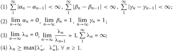
Condition 3.1
(1) ∞ 1
|αn−αn−1|<∞, ∞ 1
|βn−βn−1|<∞, ∞ 1
|γn−γn−1|<∞;
(2) nlim→∞αn= 0, lim
n→∞βn= 1, nlim→∞γn= 1;
(3)nlim→∞λn= 0, lim n→∞
λn
λn+1
= 1,∞ 1
λn=∞;
[image:4.595.132.408.630.712.2]Theorem 1[20]Under the Condition 3.1, the sequence {xn}generated by algorithm [20]converges strongly to x*ÎK, and x*is the unique solution of the VI(F, K).
We provide different conditions and establish a strong convergence theorem for the MRHSD method for variational inequalities under these conditions. Note that Condi-tion 3.2 and a strong convergence theorem (Theorem 2) are the first contribuCondi-tions of the article.
Condition 3.2
(1) 0<lim infn→∞ αn≤lim sup
n→∞ αn<1, nlim→∞βn= 1, nlim→∞γn= 1;
(2)nlim→∞λn= 0,∞ 1 λ
n=∞;
(3)λn≥max{λn, λn},∀n≥1.
Theorem 2The sequence {xn}generated by algorithm[20]converges strongly to x*Î K, and x* is the unique solution of the VI(F, K); assume that an, bn, gn and ln,λn,
λ
nsatisfy the Condition 3.2.
Proof. We divide the proof into several steps.
Step 1. [20] The sequences {xn}, {¯xn}, {˜xn} are bounded. According to Step 1, we have that
{Txn},{Tx¯n},{Tx˜n},{F(Txn)},{F(Tx¯n)},{F(Tx˜n)}}
are also bounded and xn−x∗≤M0,∀n≥0,
whereM0 = max{3∥x0 -x*∥, 3(r+g+t)∥F(x*)∥/τ}.
and
x˜n−x∗≤βnxn−x∗+ (1−βn)λn+1(γ +ρ)F(x∗)≤(1 +τ)M0, x¯n−x∗≤xn−x∗+ (1−γn)λn+1γF(x∗)≤(1 +τ)M0.
Step 2.∥xn+1-xn∥® 0.
Indeed, a series of computations yields:
¯xn− ¯xn−1=γnxn−γn−1xn−1+ (1−γn)Tλ
n+1
γ xn−(1−γn−1)Tλ
n γ xn−1 ≤ γnxn−γn−1xn−1+(1−γn)Tλ
n+1
γ xn−(1−γn−1)Tλ
n γ xn−1 ≤ xn−xn−1+(1−γn)λn+1−(1−γn−1)λnγF(Txn−1)
+|γn−γn−1|(xn−1+Txn−1).
(2)
By Tλn+1
ρ x¯n=T¯xn−λn+1 ρF(Tx¯n), Tλ
n
ρ x¯n−1=Tx¯n−1−λnρF(Tx¯n−1) and (2), we can obtain
x˜n− ˜xn−1=βnxn−βn−1xn−1+ (1−βn)Tλ
n+1
ρ x¯n−(1−βn−1)Tλ
n ρ ¯xn−1
≤ βnxn−βn−1xn−1+(1−βn)Tλ
n+1
ρ x¯n−(1−βn−1)Tλ
n ρ x¯n−1 ≤ xn−xn−1+(1−βn)λn+1−(1−βn−1)λnρF(Tx¯n−1)
+ (1−βn)(1−λn+1τ)|γn−γn−1|(xn−1+Txn−1)
+ (1−βn)(1−λn+1τ)(1−γn)λn+1 −γn−1λnγF(Txn−1)
+|βn−βn−1|(xn−1+Tx¯n−1+Tx¯n−1).
Let
˜
yn=Tλn+1t x˜n=Tx˜n−λn+1tF(Tx˜n),
so we obtain
xn+1=αnx¯n+ (1−αn)y˜n.
Furthermore,
y˜n− ˜yn−1=Tx˜n−T˜xn−1+λntF(Tx˜n−1)−λn+1tF(Tx˜n) ≤Tx˜n−Tx˜n−1+λntF(T˜xn−1)+λn+1tF(Tx˜n) ≤x˜n− ˜xn−1+λntF(Tx˜n−1)+λn+1tF(Tx˜n).
(4)
By nlim→∞βn= 1,nlim→∞λn= 0and (3), (4), we obtain: y˜n− ˜yn−1− xn−xn−1
≤(1−βn)λn+1−(1−βn−1)λnρF(Tx˜n−1)
+(1−βn)(1−λn+1τ)|γn−γn−1|(xn−1+Txn−1)
+(1−βn)(1−λn+1τ)(1−γn)λn+1 −γn−1λnγ F(Txn−1)
+|βn−βn−1|(xn−1+Tx¯n−1+Tx¯n−1)
+λntF(Tx˜n−1)+λn+1tF(Tx˜n)→0.
(5)
According to Lemma 1, we can obtain
lim
n→∞y˜n−1−xn−1= 0.
Furthermore, using the conditions nlim→∞γn= 1,maxλn,λn≤λn→0, we obtain
¯xn−xn=−(1−γn)xn+ (1−γn) Txn−λn+1γF(Txn) ≤(1−γn)xn+ (1−γn)Txn+λn+1γF(Txn)→0.
(6)
According to (5) and (6), we conclude that
xn−xn−1=αn−1x¯n−1+ (1−αn−1)˜yn−1−xn−1
≤αn−1¯xn−1−xn−1+(1−αn−1)˜yn−1−xn−1→0,
so we immediately obtain
xn+1−xn →0.
Step 3.∥xn+1-Txn∥®0.
In fact,
x˜n−xn=−(1−βn)xn+ (1−βn) Tx¯n−λn+1ρF(Tx¯n) ≤(1−βn)xn+(1−βn)Tx¯n+λn+1ρF(Tx¯n).
(7)
A series of computations yields:
xn+1−Txn=αn(x¯n−Txn)+(1−αn)
Ttλn+1x˜−Txn
≤αn¯xn−Txn+(1−αn)T˜xn−Txn
+(1−αn)λn+1tF T˜xn
≤αn¯xn−Txn+x˜n−xn+λn+1tF Tx˜ ≤αnxn+1−Txn+αn¯xn−xn+1+x˜n−xn
+λn+1tF Tx˜.
(8)
Hence, by (6), (7), (8) and Conditions 3.2, we obtain:
xn+1−Txn ≤ α n
1−αn¯
xn−xn+1+
x˜n−xn
1−αn
+λn+1tF Tx˜ 1−αn →
0. (9)
Corollary 1 ∥xn-Txn∥®0. Applying Steps 2 and 3, we get
xn+1−Txn →0
and
xn+1−xn →0,
So then
xn−Txn ≤ xn+1−Txn+xn+1−xn →0.
Step 4. lim supn→∞<−F(x∗),T˜xn−x∗>≤0.
For some x˜∈H, here exits Txni
→ ˜x weakly, and such that
lim sup
n→∞ <−F x ∗,Tx
n−x∗ >= lim sup
n→∞ <−F x ∗,Tx
ni−x∗>.
According to Txni
→ ˜x, we have
˜
x∈Fix(T)=K.
Moreover, we havex* is the unique solution ofVI(F, K), so we can obtain:
lim sup
n→∞ <−F x ∗,Tx
n−x∗>
= lim sup
n→∞ <−F x
∗,x˜−x∗>
≤0.
Since T˜xn−Txn≤˜xn−xn→0, we immediately conclude that
lim sup
n→∞ <−F x ∗,Tx˜
n−x∗>
≤lim sup
n→∞ <−F x ∗,Tx˜
n−Txn>
+ lim sup
n→∞ <−
F x∗,Txn−x∗>
≤lim sup
n→∞ <−
F x∗,Txn−x∗ >
Step 5. ∥xn- x*∥® 0. To prove this conclusion, we have to apply the Lemma 2 sev-eral times.
By Step 1 and Lemma 4, we have:
xn+1−x∗ 2
=αn x¯n−x∗
+(1−αn)
Tλn+1
t x˜n−x∗
2
≤αn x¯n−x∗2
+(1−αn)
Tλn+1
t x˜n−Tλtn+1x∗+Tλtn+1x∗−x∗
2
≤αn x¯n−x∗2+(1−αn)
Tλn+1
t ˜xn−Ttλn+1x∗
2
+2<Tλn+1
t x∗−x∗,Ttλn+1x˜n−x∗>
≤αnxn−x∗+(1−γn)λn+1γF x∗ 2
+(1−αn) (1−λn+1τ)2xn−x∗+(1−βn)λn+1(γ+ρ)F x∗2
+ 2tλn+1<−F x∗
,Tx˜n−x∗−tλn+1F Tx˜n
>
≤αnxn−x∗
2
+(1−γn)λn+1γM+(1−αn) (1−λn+1τ)2xn−x∗
2
+(1−αn) (1−λn+1τ)2(1−βn)λn+1M
+ 2tλn+1<−F x∗
,Tx˜n−x∗−tλn+1F Tx˜n
>
≤(1−(1−αn)λn+1τ)xn−x∗
2
+(1−αn)λn+1τwn+1,
(10)
where
wn+1=2t<−F(x
∗),Tx˜
n−x∗−tλn+1F Tx˜n
> τ (1−αn)
+ ϕn
τ (1−αn)
+ ξn
τ (1−αn)
,
ϕn=(1−γn) γM,
ξn=(1−αn) (1−λn+1τ)2(1−βn)M
and M0 ≪M<∞.
If we denote
sn+1=xn+1−x∗,un=(1−αn)λn+1τ,
we can rewrite (10):
sn+1≤(1−un)sn+unwn+ 0.
In fact,un, wn satisfies Lemma 2, according to
lim
n→∞βn= 1, limn→∞γn= 1, limn→∞λn= 0
and step 4, we obtain
ϕn τ (1−αn) →
0
and
ξn τ (1−αn) →
Furthermore,lim supn→∞<−F x∗,Tx˜n−x∗>≤0, so we have:
lim
n→∞
2t<−F(x∗),Tx˜n−x∗−tλn+1F Tx˜n
> τ (1−αn)
≤ 2t
τ lim supn→∞
<−F x∗,Tx˜n−x∗ >
+λn+1<−F x∗
,−tF T˜xn
> ≤ 2τtlim sup
n→∞
<−F x∗,Tx˜n−x∗>
+ lim sup
n→∞
λn+1<−F x∗
,−tF Tx˜n
>
≤0 + 0 = 0.
Consequently we obtain
lim sup
n→∞ w
n≤0,
and then from Lemma 2, we have xn−x∗→0.
which completes the proof.
The following section is our second contribution in this article.
4 Implementation of the MRHSD method for a kind of variational inequalities
Now we consider the variational inequality problem VI(F, K1 ⋂ K2), which involves
findingx*Î K1 ⋂K2 such that
x∗∈K1∩K2,<x−x∗,F x∗
>≥0,∀x∈K1∩K2, (11)
whereK1andK2are nonempty and closed convex subsets of H.
To reduce the difficulty and complexity in computing the projection PK, we solveVI (F, K1 ⋂K2) by the MRHSD method. Then we have to choose an efficient and
imple-mentable nonexpansive mapping T. Based on the spirit of the approximate projection contraction method, we define Txas:
Tx=H G(x)≈PK[x], (12)
where
G(x) =PK2(x), H(x) =PK1(x).
Assuming that PK2(x), PK1(x) can be computed without much difficulty, we can effi-ciently computeTx. According toTx≈PK[x], we can partly retain the efficiency of the projection contraction method. Obviously, the fixed point set is Fix(T) =Kand T satis-fies the property of nonexpansive mapping.
5 Numerical experiments
To show the effects of the MRHSD method for VI(F, K1 ⋂K2), we test a set of
≤HUin terms of elements. The problem considered in this section is:
min
1
2X−C
2
F|X∈K =Sn+∩ß
, (13)
where∥•∥Fis the matrix Fröbenis norm, i.e.,
CF = ⎛ ⎝∞
i=1 ∞
j=1 Cij2
⎞ ⎠ 1 2
.
Furthermore,
Sn+=H∈IRn×n|HT =H,H− 0
and
ß =H∈IRn×n|HT =H,HL≤H≤HU
.
Note that the matrix Fröbenis norm is induced by the inner product
A,B= Trace ATB.
It is known that optimization problem (13) is equivalent to the following variational inequality problem:
X−X,∇
1
2X−C
2
≥0,∀X∈K,
so we obtain
X−X,X−C≥0,∀X∈K. (14)
To solve variational inequality problem (14) by the MRHSD method, we take one set of parameter sequences satisfying Condition 3.1.
Condition 3.1.
αn=λn=λn=λn=
1
n, βn=γn= 1−
1
n, γ =ρ=t=c0>0.
Furthermore, we take two different parameter sequences satisfying Condition 3.2 to demonstrate the different effects for differentan.
Condition 3.2a.
αn= 0.3−1/(100∗n); n= 2k αn= 0.1−1/(100∗n); n= 2k−1;
λn=λn=λn= 1/(n+ 1);
βn= 1−1/n;γn= 1−1/n; n= 2k
Condition 3.2b.
αn= 0.8−1/(100∗n); n= 2k αn= 0.3−1/(100∗n); n= 2k−1;
λn=λn=λn= 1/(n+ 1);
βn= 1−1/n;γn= 1−1/n; n= 2k
βn= 1−1/n; γn= 1−1/(2n); n= 2k−1; γ =ρ=t=c0>0.
According to Tx(12), we defineTXas
TX=H(G(X)), (15)
where
G(X)= min(HU, max(X,HL)),H(X)=Psn +(X),
which can easily be computed and the fixed point set to Fix(T) = K. Moreover, according to Theorems 1 and 2, the sequences generated by algorithm [20] under Con-ditions 3.1 and 3.2 are convergent.
The computation started with ones(n, n) in MATLAB and stopped when∥xk+1 -xk∥
≤ 10-4or 10-5. All codes were implemented in MATLAB 7.0 and were run using a Pentium R 1.70 G processor on a 768 M ASUS notebook computer.
We tested the problem using n= 100, 200, 300, 400, 500. The test results for the MRHSD method under different conditions and tolerances are reported in Tables 1 and 2.
Test examples
In this example we generate the data in a similar manner as in [12]. Note that it is very difficult to compute the examples using the extended contraction method [12] when C is asymmetric. However, the MRHSD method can efficiently compute the examples whenCis asymmetric.
The diagonal elements of Care randomly generated in the interval (0, 2) and the off-diagonal elements are randomly generated in the interval (-1, 1):
(HU)jj=(HL)jj = 1,
[image:11.595.118.477.632.733.2](HU)ij=−(HL)ij= 0.1,∀i=j,i,j= 1, 2, ...,n.
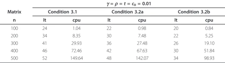
Table 1 Numerical results for tolerance of 10-4
g=r=t=c0= 0.01
Matrix Condition 3.1 Condition 3.2a Condition 3.2b
n It cpu It cpu It cpu
100 24 1.04 22 0.98 20 0.84
200 34 8.35 30 7.48 22 5.25
300 41 29.93 36 27.48 26 19.10
400 46 72.46 42 67.63 30 51.84
Matlab code:
C = zeros(n, n); HU = ones(n, n)*0.1; HL = -HU; for i = 1:n
for j = 1:n
t = mod(t*42108+13846,46273); C(i, j) = t*2/46273-1;
end; end; for i = 1:n
C(i, i) = abs(C(i, i))*2; HU(i, i) = 1; HL(i, i) = 1; end;
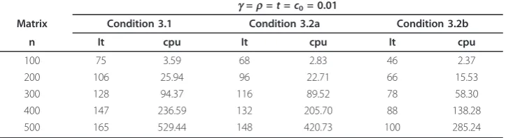
The numerical results demonstrate that this implementation of the MRHSD method is efficient. Furthermore, the MRHSD Method under Condition 3.2 is more efficient than under Condition 3.1. These numerical experiments and results are the third con-tribution of the article.
6 Conclusions and discussions
We have proved strong convergence of the MRHSD method under Condition 3.2, which differs from Condition 3.1. The proof can be simplified using Condition 3.2, which imposes suitable restrictions on the parameters. The result can be considered an improvement and refinement of previous results [20]. In particular, we designed an efficient implementation of the MRHSD method based on the approximate projection contraction method. Numerical experiments demonstrated that this is an efficient implementation and that the MRHSD method under Condition 3.2 is more efficient than under Condition 3.1. However, choosing an efficient and implementable nonex-pansive mapping for a generalVI(F, K) is still a difficult problem.
Acknowledgements
This research was supported by National Science and Technology Support Program (Grant No. 2011BAH24B06), Science Foundation of the Civil Aviation Flight University of China (Grant No. J2010-45).
Author details
1School of Civil Aviation, Nanjing University of Aeronautics and Astronautics, Nanjing 210016, China2School of Computer Science, Civil Aviation Flight University of China, Guanghan 618307, China
Competing interests
The author declares that they have no competing interests.
[image:12.595.118.480.103.202.2]Received: 1 October 2011 Accepted: 19 April 2012 Published: 19 April 2012
Table 2 Numerical results for tolerance of 10-5
g=r=t=c0= 0.01
Matrix Condition 3.1 Condition 3.2a Condition 3.2b
n It cpu It cpu It cpu
100 75 3.59 68 2.83 46 2.37
200 106 25.94 96 22.71 66 15.53
300 128 94.37 116 89.52 78 58.30
400 147 236.59 132 205.70 88 138.28
References
1. Hartman, P, Stampacchia, G: On some nonlinear elliptic differential functional equations. Acta Math.115, 153–188 (1966)
2. Stampacchia, G: Variational inequalities in theory and applications of monotone operators. Proceedings of the NATO Advanced Study Institute. pp. 102–192.Venice, Italy(Edizioni Oderisi, Gubbio, Italy) (1968)
3. Harker, PT, Pang, JS: Finite-dimensional variational inequality and nonlinear complementarity problems: a survey of theory, algorithms and applications. Math Program.48, 161–220 (1990)
4. Smith, MJ: The existence, uniqueness and stability of traffic equilibria. Transport Res.13B, 295–304 (1979)
5. Mathiesen, L: Computation of economic equilibria by a sequence of linear complementarity problems. Math Program Stud.23, 144–162 (1985)
6. Huang, NJ, Li, J, Wu, SY: Optimality conditions for vector optimization problems. J Optim Theory Appl.142, 323–342 (2009)
7. Deutsch, F, Yamada, I: Minimizing certain convex functions over the intersection of the fixed-point sets of nonexpansive mappings. Numer Func Anal Opt.19, 33–56 (1998)
8. Yamada, I: The hybrid steepest-descent method for variational inequality problems over the intersection of the fixed-point sets of nonexpansive mappings. Stud Comput Math.8, 473–504 (2001)
9. Xu, HK, Kim, TH: Convergence of hybrid steepest-descent methods for variational inequalities. J Optim Theory Appl.
119, 185–201 (2003)
10. Zeng, LC, Wong, NC, Yao, JC: Convergence analysis of modified hybrid steepest-descent methods with variable parameters for variational inequalities. J Optim Theory Appl.132, 51–69 (2007)
11. Ding, XP, Lin, YC, Yao, JC: Three-step relaxed hybrid steepest-descent methods for variational inequalities. Appl Math Mech.28, 1029–1036 (2007)
12. He, BS, Liao, LZ, Wang, X: Proximal-like contraction methods for monotone variational inequalities in a unified framework. http://www.optimization-online.org/DB-HTML/2008/12/2163.html (2009). doi:10.1007/s10589-010-9372-0 13. He, BS, Yang, ZH, Yuan, XM: An approximate proximal-extragradient type method for monotone variational inequalities.
J Math Anal Appl.300, 362–374 (2004)
14. He, BS: A new method for a class of linear variational inequalities. Math Program.66, 137–144 (1994)
15. He, BS: A class of projection and contraction methods for monotone variational inequalities. Appl Math Optim.35, 69–76 (1997)
16. Li, M, Bnouhachem, A: A modified inexact operator splitting method for monotone variational inequalities. J Glob Optim.41, 417–426 (2008)
17. Sun, DF: A projection and contraction method for the nonlinear complementarity problem and its extensions. Math Numer Sin.16, 183–194 (1994)
18. Noor, MA: New approximation schemes for general variational inequalities. J Math Anal Appl.251, 217–229 (2005) 19. Yao, YH, Noor, MA, Chen, RD, Liou, YC: Strong convergence of three-step relaxed hybrid steepest-descent methods for
variational inequalities. Appl Math Comput.201, 175–183 (2008)
20. Xu, HW, Song, EB, Pan, HP, Shao, H, Sun, LM: The modified and relaxed hybrid steepest-descent methods for variational inequalities. In Proceedings of the 1st International Conference on Modelling and Simulation, vol. II, pp. 169–174.World Academic Press (2008)
21. Suzuki, T: Strong convergence of Krasnoselskii and Mann’s type sequences for one-parameter nonexpansive semigroups without Bochner integrals. J Math Anal Appl.305, 227–239 (2005)
22. Gao, Y, Sun, DF: Calibrating least squares covariance matrix problems with equality and inequality constraints. http:// www.math.nus.edu.sg/matsundf/CaliMat_June_2008.pdf (2008)
doi:10.1186/1029-242X-2012-93
Cite this article as:Xu:Efficient implementation of a modified and relaxed hybrid steepest-descent method for a type of variational inequality.Journal of Inequalities and Applications20122012:93.
Submit your manuscript to a
journal and benefi t from:
7Convenient online submission 7Rigorous peer review
7Immediate publication on acceptance 7Open access: articles freely available online 7High visibility within the fi eld
7Retaining the copyright to your article