A New Projection Algorithm for Generalized Variational Inequality

Volume 2010, Article ID 182576,8pages doi:10.1155/2010/182576

Research Article

A New Projection Algorithm for Generalized

Variational Inequality

Changjie Fang

_{and Yiran He}

1_{Department of Mathematics, Sichuan Normal University, Chengdu, Sichuan 610068, China} 2_{Institute of Applied Mathematics, Chongqing University of Posts and Telecommunications,}

Chongqing 400065, China

Correspondence should be addressed to Changjie Fang,[email protected]

Received 26 October 2009; Accepted 20 December 2009

Academic Editor: Vy Khoi Le

Copyrightq2010 C. Fang and Y. He. This is an open access article distributed under the Creative Commons Attribution License, which permits unrestricted use, distribution, and reproduction in any medium, provided the original work is properly cited.

We propose a new projection algorithm for generalized variational inequality with multivalued mapping. Our method is proven to be globally convergent to a solution of the variational inequality problem, provided that the multivalued mapping is continuous and pseudomonotone with nonempty compact convex values. Preliminary computational experience is also reported.

1. Introduction

We consider the following generalized variational inequality. To findx∗ ∈ Candξ ∈ Fx∗ such that

ξ, y−x∗_{≥0, ∀y∈C, 1.1}

whereC is a nonempty closed convex set inRn, F is a multivalued mapping fromC into Rn _{with nonempty values, and·,· and · denote the inner product and norm in R}n_,

respectively.

the literature; see 14–17 and the references therein. Recently, 15 proposes a projection algorithm for generalized variational inequality with pseudomonotone mapping. In 15, choosing ξi ∈ Fxi needs solving a single-valued variational inequality and hence is

computationally expensive; see expression2.1in15. In this paper, we introduce a different projection algorithm for generalized variational inequality. In our method, ξi ∈ Fxi can

be taken arbitrarily. Moreover, the main difference of our method from that of15 is the procedure of Armijo-type linesearch; see expression2.2in15and expression2.2in the next section.

Let S be the solution set of 1.1, that is, those points x∗ ∈ C satisfying 1.1. Throughout this paper, we assume that the solution setSof problem1.1is nonempty andF is continuous onCwith nonempty compact convex values satisfying the following property:

ζ, y−x≥0, ∀y∈C, ζ∈Fy, ∀x∈S. 1.2

Property 1.2 holds if F is pseudomonotone on C in the sense of Karamardian 18. In particular, ifFis monotone, then1.2holds.

The organization of this paper is as follows. In the next section, we recall the definition of continuous multivalued mapping, present the algorithm details, and prove the preliminary result for convergence analysis inSection 3. Numerical results are reported in the last section.

2. Algorithms

Let us recall the definition of continuous multivalued mapping. F is said to be upper semicontinuous at x ∈ Cif for every open set V containing Fx, there is an open setU containingx such thatFy ⊂ V for ally ∈ C ∩ U. F is said to be lower semicontinuous at x ∈ C, if we give any sequence xk converging to x and any y ∈ Fx, there exists a

sequencey_k ∈ Fx_kthat converges toy.F is said to be continuous at x ∈ C if it is both upper semicontinuous and lower semicontinuous atx. IfFis single valued, then both upper semicontinuity and lower semicontinuity reduce to the continuity ofF.

LetΠCdenote the projector ontoCand letμ >0 be a parameter.

Proposition 2.1. x∈Candξ∈Fxsolve problem1.1if and only if

rμx, ξ:x−ΠCx−μξ0. 2.1

Algorithm 2.2. Choosex0∈Cand three parametersσ >0, 0< μ < min{1,1/σ}, andγ∈0,1.

Seti0.

Step 1. Ifrμxi, ξ 0 for someξ∈Fxi, stop; else take arbitrarilyξi∈Fxi.

Step 2. Letk_ibe the smallest nonnegative integer satisfying

ξi−yi, rμxi, ξi≤σrμxi, ξi2, 2.2

Step 3. Computexi 1: ΠCixi,whereCi:{x∈C:hix≤0}, and

hix:yi ηirμxi, ξi, x−xi ηiyi−μξi rμxi, ξi, rμxi, ξi. 2.3

Leti:i 1 and go toStep 1.

Remark 2.3. SinceFhas compact convex values,F has closed convex values. Therefore,y_iin Step 2is uniquely determined byki.

Remark 2.4. If F is a single-valued mapping, the Armijo-type linesearch procedure 2.2 becomes that ofAlgorithm 2.2in14.

We show thatAlgorithm 2.2is well defined and implementable.

Proposition 2.5. Ifxi is not a solution of problem1.1, then there exists a nonnegative integerki

satisfying2.2.

Proof. Suppose that for allk, we have

ξi−yk, rμxi, ξi> σrμxi, ξi2, 2.4

where yk ΠFxi−γkrμxi,ξiξi. Since F is lower semicontinuous, ξi ∈ Fxi, and xi − γk_{rμxi, ξi → xi as k → ∞, for each k, there is uk ∈ Fxi − γ}k_{rμxi, ξi such that}

limk→ ∞ukξi. Sinceyk ΠFxi−γkrμxi,ξiξi,

_{yk−ξi≤ uk−ξi −→}0, ask−→ ∞. 2.5

So limk→ ∞yk ξi. Let k → ∞ in 2.4, we have 0 ξi −ξi ≥ σrμxi, ξi > 0. This

contradiction completes the proof.

Lemma 2.6. For everyx∈Candξ∈Fx,

ξ, rμx, ξ≥μ−1rμx, ξ2. 2.6

Proof. See15, Lemma 2.3.

Lemma 2.7. Let C be a closed convex set inRn, ha real-valued function on Rn, and K the set

{x∈C:hx≤0}. IfKis nonempty andhis Lipschitz continuous onCwith modulusθ >0, then

distx, K≥θ−1_{max{hx,0}, ∀x∈C, 2.7}

wheredistx, Kdenotes the distance fromxtoK.

Proof. See14, Lemma 2.3.

Lemma 2.8. Letx∗solve the variational inequality1.1and let the functionhibe defined by2.3.

Thenh_ix_i≥η_iμ−1−σr_μx_i, ξ_i2_andh

Proof. It follows from2.3that

hixi ηiyi−μξi rμxi, ξi, rμxi, ξi

ηiyi, rμxi, ξi−μηiξi, rμxi, ξi ηirμxi, ξi2

≥ηi1−μξi, rμxi, ξi ηi1−σrμxi, ξi2

≥μ−1_−ση

irμxi, ξi2,

2.8

where the first inequality follows from2.2and the last one follows from Lemma 2.6and μ <1. Ifr_μx_i, ξ_i/0, thenh_ix_i>0 becauseμ <1/σ. It remains to be proved thath_ix∗≤0. Sincerμxi, ξi xi−ΠCxi−μξi, we have

rμxi, ξi−μξi, x∗−xi rμxi, ξi≤0, 2.9

on the other hand, assumption1.2implies that

μξi, x∗−xiμξi, x∗−xi ≤0. 2.10

Adding the last two expressions, we obtain that

rμxi, ξi, x∗−xi≤rμxi, ξi, μξi−rμxi, ξi. 2.11

It follows that

yi ηirμxi, ξi, x∗−xiyi, x∗−xi ηirμxi, ξi, x∗−xi ≤yi, x∗−xi ηirμxi, ξi, μξi−rμxi, ξi

yi, x∗−xi ηirμxi, ξi−ηiyi−μξi rμxi, ξi, rμxi, ξi ≤ −ηiyi−μξi rμxi, ξi, rμxi, ξi,

2.12

where the second inequality follows from assumption1.2andyi∈Fxi−ηirμxi, ξi. Thus

hix∗≤0 is verified.

3. Main Results

Proof. Letx∗be a solution of the variational inequality problem. ByLemma 2.8,x∗ ∈Ci. We

assume thatAlgorithm 2.2generates an infinite sequence{x_i}. In particular,r_μx_i, ξ_i/0 for everyi. ByStep 3, it follows from Lemma 2.4 in14that

xi 1−x∗2≤ xi−x∗2− xi 1−xi2≤ xi−x∗2−dist2xi, Ci, 3.1

where the last inequality is due to xi 1 ∈ Ci. It follows that the squence {xi 1−x∗2} is

nonincreasing, and hence is a convergent sequence. Therefore,{x_i}is bounded and

lim

i→ ∞dist 2_x

i, Ci 0. 3.2

By the boundedness of{x_i}, there exists a convergent subsequence{x_ij}converging tox. If x is a solution of problem 1.1, we show next that the whole sequence {xi} converges tox. Replacingx∗ byxin the preceding argument, we obtain that the sequence

{xi−x} is nonincreasing and hence converges. Sincexis an accumulation point of{xi},

some subsequence of {xi −x} converges to zero. This shows that the whole sequence {xi−x}converges to zero, hence limi→ ∞xi x.

Suppose now that x is not a solution of problem 1.1. We show first that k_i in Algorithm 2.2cannot tend to∞. SinceFis continuous with compact values, Proposition 3.11 in19implies that {Fxi : i ∈N}is a bounded set, and so the sequence{ξi}is bounded.

Therefore, there exists a subsequence{ξ_ij} converging toξ. SinceFis upper semicontinuous with compact values, Proposition 3.7 in19implies thatFis closed, and soξ ∈Fx. By the definition ofki, we have

ξi−ui, rμxi, ξi> σrμxi, ξi2, ∀ui ΠFxi−γki−1rμxi,ξiξi. 3.3

If kij → ∞, then xij −γkij−1rμxij, ξij → x. The lower continuity of F, in turn, implies

the existence of ξ_ij ∈ Fx_ij − γkij−1_r

μxij, ξij such that ξij converges to ξ. Since uij

Π_Fx

ij−γkij−1rμxij,ξijξij, uij ∈ Fxij −γ

kij−1_r

μxij, ξij, and uij −ξij ≤ ξij −ξij. Therefore

limj→ ∞uij ξand

ξij−uij, rμ

xij, ξij

> σrμ

xij, ξij 2

. 3.4

Lettingj → ∞, we obtain the contradiction

0≥σrμ

x, ξ2>0, 3.5

It follows from2.3that

_hix−hi

yyi ηirμxi, ξi, x−y≤yi ηirμxi, ξix−y. 3.6

Since{xi}and {ξi}are bounded, we have the sequence{rμxi, ξi}and hence the sequence {Fxi−ηirμxi, ξi}is bounded. Thus, for someM >0,

_{yi ηirμxi, ξi≤ sup}

ζ∈Fxi−ηirμxi,ξi

ζ ηirμxi, ξi≤M, ∀i. _3.7

Therefore, each functionhiis Lipschitz continuous onCwith modulusM. Noting thatxi/∈Ci

and applyingLemma 2.7, we obtain that

distxi, Ci≥M−1hixi, ∀i. 3.8

It follows from3.8andLemma 2.8that

distxi, Ci≥M−1hixi≥M−1

μ−1_−ση

irμxi, ξi2. 3.9

Then3.2implies that

lim

i→ ∞ηirμxi, ξi 2

0. 3.10

By the boundedness of{ηi}, we obtain that limi→ ∞rμxi, ξi0.Sincerμ·,·is continuous

and the sequences {xi} and {ξi} are bounded, there exists an accumulation point x, ξ of

{xi, ξi} such that rμx, ξ 0. This implies thatx solves the variational inequality1.1.

Similar to the preceding proof, we obtain that limi→ ∞xix.

4. Numerical Experiments

In this section, we present some numerical experiments for the proposed algorithm. The MATLAB codes are run on a PC with CPU Intel P-T2390 under MATLAB Version 7.0.1.24704R14Service Pack 1. We compare the performance of ourAlgorithm 2.2and15, Algorithm1. In the Tables1and2, “It.” denotes number of iteration, and “CPU” denotes the CPU time in seconds. The toleranceεmeans whenrx, ξ ≤ε,the procedure stops.

Example 4.1. Letn3,

C:

x∈Rn_:n i1

xi1

, 4.1

and letF:C → 2Rn be defined by

Table 1:Example 4.1.

Algorithm 2.2 15, Algorithm 1

ε It.num. CPUsec. It.num. CPUsec.

10−7 55 0.625 74 0.984375

10−5 39 0.546875 51 0.75

10−3 23 0.4375 27 0.5

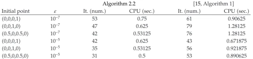
Table 2:Example 4.2.

Algorithm 2.2 15, Algorithm 1

Initial point ε It.num. CPUsec. It.num. CPUsec.

0,0,0,1 10−7 53 0.75 61 0.90625

0,0,1,0 10−7 47 0.625 79 1.28125

0.5,0,0.5,0 10−7 _{42 0.53125 76 1.28125}

0,0,0,1 10−5 42 0.625 43 0.671875

0,0,1,0 10−5 35 0.53125 56 0.921875

0.5,0,0.5,0 10−5 31 0.5 53 0.890625

Then the setCand the mapping F satisfy the assumptions ofTheorem 3.1and0,0,1is a solution of the generalized variational inequality. Example 4.1is tested in 15. We choose σ 0.5, γ 0.8, andμ 1 for our algorithm;σ 0.8, γ 0.6, andμ 1 for Algorithm1in 15. We usex0 0.3,0.4,0.3as the initial point.

Example 4.2. Letn4,

C:

x∈Rn_:n i1

xi1

, 4.3

andF:C → 2Rn be defined by

Fx {t, t 2x2, t 3x3, t 4x4:t∈0,1}. 4.4

Then the setCand the mappingF satisfy the assumptions ofTheorem 3.1and1,0,0,0is a solution of the generalized variational inequality. We chooseσ 0.5, γ 0.8, andμ 1 for the two algorithms.

Acknowledgments

References

1 E. Allevi, A. Gnudi, and I. V. Konnov, “The proximal point method for nonmonotone variational inequalities,”Mathematical Methods of Operations Research, vol. 63, no. 3, pp. 553–565, 2006.

2 A. Auslender and M. Teboulle, “Lagrangian duality and related multiplier methods for variational inequality problems,”SIAM Journal on Optimization, vol. 10, no. 4, pp. 1097–1115, 2000.

3 T. Q. Bao and P. Q. Khanh, “A projection-type algorithm for pseudomonotone nonlipschitzian mul-tivalued variational inequalities,” inGeneralized Convexity, Generalized Monotonicity and Applications, vol. 77 ofNonconvex Optimization and Its Applications, pp. 113–129, Springer, New York, NY, USA, 2005. 4 L. C. Ceng, G. Mastroeni, and J. C. Yao, “An inexact proximal-type method for the generalized variational inequality in Banach spaces,”Journal of Inequalities and Applications, vol. 2007, Article ID 78124, 14 pages, 2007.

5 S. C. Fang and E. L. Peterson, “Generalized variational inequalities,”Journal of Optimization Theory and Applications, vol. 38, no. 3, pp. 363–383, 1982.

6 M. Fukushima, “The primal Douglas-Rachford splitting algorithm for a class of monotone mappings with application to the traffic equilibrium problem,”Mathematical Programming, vol. 72, no. 1, pp. 1–15, 1996.

7 Y. He, “Stable pseudomonotone variational inequality in reflexive Banach spaces,” Journal of Mathematical Analysis and Applications, vol. 330, no. 1, pp. 352–363, 2007.

8 R. Saigal, “Extension of the generalized complementarity problem,” Mathematics of Operations Research, vol. 1, no. 3, pp. 260–266, 1976.

9 G. Salmon, J.-J. Strodiot, and V. H. Nguyen, “A bundle method for solving variational inequalities,”

SIAM Journal on Optimization, vol. 14, no. 3, pp. 869–893, 2003.

10 R. T. Rockafellar, “Monotone operators and the proximal point algorithm,”SIAM Journal on Control and Optimization, vol. 14, no. 5, pp. 877–898, 1976.

11 I. V. Konnov, “On the rate of convergence of combined relaxation methods,” Izvestiya Vysshikh Uchebnykh Zavedenii. Matematika, no. 12, pp. 89–92, 1993.

12 I. V. Konnov, Combined Relaxation Methods for Variational Inequalities, vol. 495 of Lecture Notes in Economics and Mathematical Systems, Springer, Berlin, Germany, 2001.

13 I. V. Konnov, “Combined relaxation methods for generalized monotone variational inequalities,” in

Generalized Convexity and Related Topics, vol. 583 ofLecture Notes in Econom. and Math. Systems, pp. 3–31, Springer, Berlin, Germany, 2007.

14 Y. He, “A new double projection algorithm for variational inequalities,”Journal of Computational and Applied Mathematics, vol. 185, no. 1, pp. 166–173, 2006.

15 F. Li and Y. He, “An algorithm for generalized variational inequality with pseudomonotone mapping,”Journal of Computational and Applied Mathematics, vol. 228, no. 1, pp. 212–218, 2009. 16 M. V. Solodov and B. F. Svaiter, “A new projection method for variational inequality problems,”SIAM

Journal on Control and Optimization, vol. 37, no. 3, pp. 765–776, 1999.

17 F. Facchinei and J. S. Pang,Finite-Dimensional Variational Inequalities and Complementary Problems, Springer, New York, NY, USA, 2003.

18 S. Karamardian, “Complementarity problems over cones with monotone and pseudomonotone maps,”Journal of Optimization Theory and Applications, vol. 18, no. 4, pp. 445–454, 1976.