Volume 2009, Article ID 965712,13pages doi:10.1155/2009/965712
Research Article
The Kolmogorov Distance between
the Binomial and Poisson Laws: Efficient
Algorithms and Sharp Estimates
Jos ´e A. Adell, Jos ´e M. Anoz, and Alberto Lekuona
Departamento de M´etodos Estad´ısticos, Facultad de Ciencias, Universidad de Zaragoza, 50009 Zaragoza, Spain
Correspondence should be addressed to Jos´e A. Adell,[email protected]
Received 21 May 2009; Accepted 9 October 2009
Recommended by Andrei Volodin
We give efficient algorithms, as well as sharp estimates, to compute the Kolmogorov distance between the binomial and Poisson laws with the same meanλ. Such a distance is eventually attained at the integer part ofλ1/2−λ1/4. The exact Kolmogorov distance forλ≤2−√2 is also provided. The preceding results are obtained as a concrete application of a general method involving a differential calculus for linear operators represented by stochastic processes.
Copyrightq2009 Jos´e A. Adell et al. This is an open access article distributed under the Creative Commons Attribution License, which permits unrestricted use, distribution, and reproduction in any medium, provided the original work is properly cited.
1. Introduction and Main Results
The aim of this paper is to obtain efficient algorithms and sharp estimates in the highly classical problem of evaluating the Kolmogorov distance between binomial and Poisson laws having the same mean. The techniques used here are analogous to those in2dealing with the total variation distance between the aforementioned laws.
To state our main results, let us introduce some notation. Denote by Z the set of
nonnegative integers,NZ\ {0}andZn {0,1, . . . , n},n∈N. IfAis a set of real numbers, 1A stands for the indicator function ofA. For anyx ≥0, we setx max{k ∈ Z : k ≤ x}
andx min{k ∈Z : x≤ k}. For anym ∈Z, themth forward differences of a function
φ : Z → R are recursively defined by Δ0φ φ, Δ1φ i φ i1−φ i,i ∈ Z
, and
Δm1φ Δ1 Δmφ.
Throughout this note, it will be assumed thatn ∈ N, 0 < λ < n, and p λ/n. Let Uk, k ∈ Nbe a sequence of independent identically distributed random variables having the uniform distribution on0,1. The random variable
Sn t n
k1
10,t Uk, 0≤t≤1, S0 t≡0, 1.1
has the binomial distribution with parametersnandt. LetNλbe a random variable having the Poisson distribution with mean λ. Recall that the Kolmogorov distance betweenSn p andNλis defined by
dSn
p, Nλ
sup i∈Z
f i, f i P Nλ≥i−P Sn
p≥i, i∈Z. 1.2
Observe that for anyi∈Znwe have
Δ1f i PS
n
pi−P Nλi P Nλi
c n, λ
gn,λ i − 1
, 1.3
where
c n, λ n!eλ
1− λ n
n
, gn,λ i n−i! n−λi. 1.4
An efficient algorithm to computed Sn p, Nλis based on the zeroes of the second Krawtchouk and Charlier polynomials, which are the orthogonal polynomials with respect to the binomial and Poisson distributions, respectively. Interesting references for general orthogonal polynomials are the monographs by Chihara5and Schoutens6.
More precisely, letk∈Nwithk≥n, and 0< t <1. The second Krawtchouk polynomial with respect toSk1 tis given by
Q2k1 t;x x
2− 12ktxk k1t2
The two zeroes of this polynomial are
xjk1 t 1
2kt −1
j kt 1−t 1
4, j 1,2. 1.6
Ask → ∞,t → 0, andkt → λ,Q2k1 t;xconverges to the second Charlier polynomial with respect toNλdefined by
C2 λ;x x
2− 12λxλ2
λ2 , 1.7
the two zeroes of which are
rj λ 1
2λ −1
j λ1
4, j 1,2. 1.8
Finally, we denote by
r1,k λ x1k1
λ k
1
2 λ− λ
1−λ k
1
4, 1.9
and by
r2,k λ x2k1
λ k1
1
2 λ k
k1 λ
1− λ
k1
k k1
1
4 1.10
the smallest zero ofQ2k1 λ/k;xand the greatest zero ofQ2k1 λ/ k1;x, respectively, seeFigure 1.
Our first main result is the following.
Theorem 1.1. Letn∈Nand0< λ < n. Then,
dSn
p, Nλ
max−f lλ n, f mλ n 1
, 1.11
wherefis defined in 1.2,
lλ n min
i∈r1 λ1,r1,n λ ∩Zn;gn,λ i≤c n, λ
, 1.12
mλ n max
i∈r2,n λ,r2 λ −1∩Zn;gn,λ i≤c n, λ
. 1.13
Looking at Figure 1 and taking into account 1.8, 1.9, and 1.12 we see the following. The number of computations needed to evaluatelλ nis approximatelyr1,n λ− r1 λ, that is, λ
√
Q2k1 λ k;x
Q2k1 λ k1;x
C2λ;x
r2λ
r2,kλ r1,k λ
[image:4.600.210.389.99.268.2]r1λ
Figure 1:The polynomialsQ2k1λ/k;x,Q2k1 λ/k1;x, andC2 λ;x, forλ >2.
approximates Sn p if and only if p λ/n is close to zero. Moreover, the set r1 λ
1,r1,n λ ∩Znhas two points at most, wheneverr1,n λ−r1 λ<1, and this happens if
n > λ
2
√
4λ5−2. 1.14
As follows from 1.2, the natural way to compute the Kolmogorov distance
d Sn p, Nλis to look at the maximum absolute value of the function
f i i−1 k0
Δ1f k i−1
k0
PSn
pk−P Nλk
, i∈N. 1.15
From a computational point of view, the main question is to ask how many evaluations of the probability differencesP Sn p k−P Nλ k are required to exactly compute d Sn p, Nλ. According toTheorem 1.1and 1.8, the number of such evaluations isλ−
√ λ at least, andλ√λat most, approximately.
On the other hand, r1,n λand r2,n λ converge, respectively, to r1 λand r2 λ, as
n → ∞. Thus,Theorem 1.1leads us to the following asymptotic result.
Corollary 1.2. Letn ∈ Nand0 < λ < n. Letn0 λbe the smallest integer such thatr1,n λ
r1 λ1andr2,n λr2 λ −1, forn≥n0 λ. Then, one has for anyn≥n0 λ
dSn
p, Nλ
maxP Nλ≤ r1 λ−P
Sn
p≤ r1 λ
,
PSn
p≤ r2 λ
−P Nλ≤ r2 λ
.
1.16
Unfortunately,n0 λis not uniformly bounded whenλvaries in an arbitrary compact
set. In fact, sincer1 l
√
l l,l ∈ N, andr2 m−√m m,m 2,3, . . ., it can be verified
thatn0 λ → ∞, whenλ → l
√
right,m2,3, . . . .This explains whylλ nandmλ ninTheorem 1.1have no simple form in general.
Finally, it may be of interest to compare Theorem 1.1 and Corollary 1.2 with the exact value of the Kolmogorov distance in the central limit theorem for symmetric binomial distributions obtained by Hipp and Mattner 4. These authors have shown that cf. 4, Corollary 1.1
d
Sn 1/2 −n/2
n/4 , Z
⎧ ⎪ ⎪ ⎪ ⎨ ⎪ ⎪ ⎪ ⎩ P Z≤ √1
n
−1
2 nodd,
1 2P Sn 1 2 n 2 neven, 1.17
whereZ is a standard normal random variable. Roughly speaking, 1.17tells us that the Kolmogorov distance in this version of the central limit theorem is attained at the mean of the respective distributions; whereas according to Theorem 1.1 and Corollary 1.2, the Kolmogorov distance in our Poisson approximation setting is attained at the mean ± the standard deviation of the corresponding distributions.
For small values ofλ, we are able to give the following closed-form expression.
Corollary 1.3. Letn∈N. If0< λ≤2−√2, then
dSn
p, Nλ
P Nλ0−P
Sn
p0e−λ−
1−λ n
n
. 1.18
Corollary 1.3can be seen as a counterpart of the total variation result established by Kennedy and Quine1, Theorem 1, stating that
dTV
Sn
p, Nλ
PSn
p1−P Nλ1 λ
1− λ n
n−1
−e−λ
, 1.19
for anyn∈Nand 0< λ≤2−√2, wheredTV ·,·stands for the total variation distance.
For anym∈N,n2,3, . . ., and 0< λ < n, we denote by
Kλ n n2 2 n1
2λ
3 f3 n, λ λ2
4 f4 n, λ
, 1.20
where
fm n, λ min
2m−1,1 2
n2 n−1
3/2 m!
λm 1− λ/nm
. 1.21
Theorem 1.4. Letn2,3, . . .,0< λ < nandpλ/n. Then,
dSn
p, Nλ
−1
2pMλ
≤Kλ np2, 1.22
where
Mλe−λ
λr1λ λ− r1 λ r1 λ!
. 1.23
Upper bounds for the Kolmogorov distance in Poisson approximation for sums of independent random indicators have been obtained by many authors using different techniques. We mention the following estimates in the case at hand:
dSn
p, Nλ
≤ 1
2λp 1.24
Serfling7,
dSn
p, Nλ
≤ π
4p 1.25
Hipp8,
dSn
p, Nλ
−1
2pmax
Mλ,Mλ
≤
1 2
π
8
p3/2
1− √p 1.26
Deheuvels et al.9,
dSn
p, Nλ
≤ 1 2ep
6p3/2
51− √p 1.27
Roos10, where
Mλe−λ
λr2λ r2 λ −λ r2 λ!
, 1.28
and the constant 1/ 2ein the last estimate is best possible cf. Roos10. It is readily seen
from 1.23that
lim λ→ ∞Mλ
1 √
2πe, Mλλe
−λ, 0< λ <2. 1.29
On the other hand, it follows from Roos10andLemma 2.1below that
Mλ≤Mλ≤M1 1
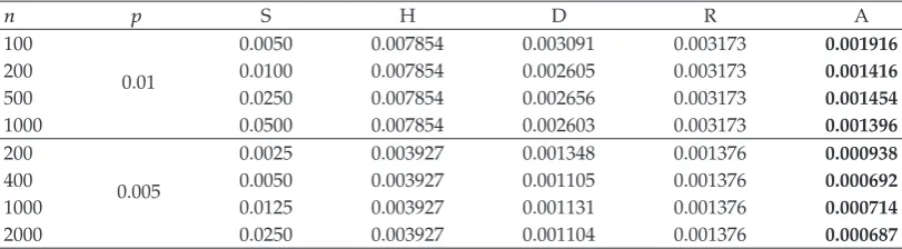
Table 1:Upper bounds fordSn p, Nλ: Serfling S, Hipp H, Deheuvels et al. D, Roos R, and Adell et al. A.
n p S H D R A
100
0.01
0.0050 0.007854 0.003091 0.003173 0.001916 200 0.0100 0.007854 0.002605 0.003173 0.001416
500 0.0250 0.007854 0.002656 0.003173 0.001454 1000 0.0500 0.007854 0.002603 0.003173 0.001396 200
0.005
0.0025 0.003927 0.001348 0.001376 0.000938 400 0.0050 0.003927 0.001105 0.001376 0.000692 1000 0.0125 0.003927 0.001131 0.001376 0.000714 2000 0.0250 0.003927 0.001104 0.001376 0.000687
Such properties, together with simple numerical computations performed with MapleTM9.01,
show that estimate 1.22is always better than the preceding ones for 0< p≤1/3 andn≥10. Numerical comparisons are exhibited inTable 1.
On the other hand, the referee has drawn our attention to a recent paper by Vaggelatou 11, where the author obtains upper bounds for the Kolmogorov distance between sums of
independent integer-valued random variables. Specializing Corollary 15 in11to the case at hand, Vaggelatou gives the upper bound
dSn
p, Nλ
≤ Mλ
2 1−2 1−e−pp λ2
2 p
2. 1.31
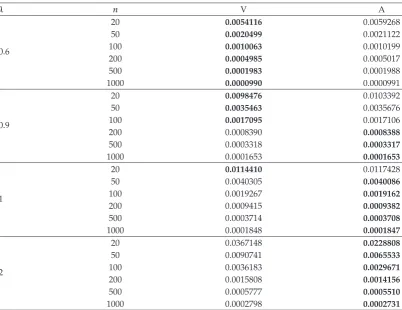
ComparingCorollary 1.3and 1.22with 1.31, we see the following. The constant in
the main term of the order ofpin 1.22is better than that in 1.31. The constantKλ nin the remainder term of the order ofp2in 1.22is uniformly bounded inλ, whereas;λ2/2 is not.
However,λ2/2 is better thanK
λ nfor small values ofλ > 2− √
2 recall thatCorollary 1.3
gives the exact distance for 0 < λ ≤ 2−√2. As a result, for moderate or large values ofn, estimate 1.31is sometimes better than 1.22for 2−√2< λ <1, approximately. Otherwise,
Corollary 1.3and 1.22provide better bounds than 1.31. This is illustrated inTable 2. We finally establish that, for small values ofp, the Kolmogorov distance is attained at r1 λ, that is, atλ−
√
λ, approximately. This completes the statement inCorollary 1.3.
Corollary 1.5. For anyλ >0, one has
lim p→0
1 pd
Sn
p, Nλ
lim
p→0
1 p
P Nλ≤ r1 λ−P
Sn
p≤ r1 λ
Mλ
2 . 1.32
Remark 1.6. As far as upper bounds are concerned, the methods used in this paper can be adapted to cover more general cases referring to Poisson approximation see, e.g., the Introduction in2and the references therein. However, the obtention of efficient algorithms
leading to exact values is a more delicate question. As we will see in Section 2, specially in formula 2.1, such a problem is based on two main facts: first, the explicit form of the
Table 2:Upper bounds fordSn p, Nλ: Vaggelatou Vand Adell et al. A.
λ n V A
0.6
20 0.0054116 0.0059268
50 0.0020499 0.0021122
100 0.0010063 0.0010199
200 0.0004985 0.0005017
500 0.0001983 0.0001988
1000 0.0000990 0.0000991
0.9
20 0.0098476 0.0103392
50 0.0035463 0.0035676
100 0.0017095 0.0017106
200 0.0008390 0.0008388
500 0.0003318 0.0003317
1000 0.0001653 0.0001653
1
20 0.0114410 0.0117428
50 0.0040305 0.0040086
100 0.0019267 0.0019162
200 0.0009415 0.0009382
500 0.0003714 0.0003708
1000 0.0001848 0.0001847
2
20 0.0367148 0.0228808
50 0.0090741 0.0065533
100 0.0036183 0.0029671
200 0.0015808 0.0014156
500 0.0005777 0.0005510
1000 0.0002798 0.0002731
these orthogonal polynomials. For instance, an explicit expression for the orthogonal polynomials associated to general sums of independent random indicators seems to be unknown.
2. The Proofs
The key tool to prove the previous results is the following formula established in2, formula 1.4. For any functionφ:Z → Rfor which the expectations below exist, we have
EφSn
p−Eφ Nλ −λ2 ∞
kn 1
k k1EUΔ2φ Sk−1 Tk
−λ2 ∞
kn 1
k k1EUφ Sk1 TkQ2k1 Tk;Sk1 Tk,
2.1
where
Tk λ k
1− UV
k1
andUandV are independent identically distributed random variables having the uniform distribution on0,1, also independent of the sequence Uk, k∈Nin 1.1.
Proof ofTheorem 1.1. Letn ∈ N, 0 < λ < n, andi ∈ Z. The functiongn,λ idefined in 1.4 decreases in0,λ1∩Zn and increases inλ1, n∩Zn. This property, together with definitions 1.2– 1.4, readily implies the following. There are integers 1≤lλ n≤mλ n≤n such that
i∈Zn;gn,λ i≤c n, λ
i∈Z:Δ1f i≥0 lλ n, mλ n∩Zn. 2.3
As a consequence of 2.3, the functionf idefined in 1.2starts fromf 0 0, decreases in0, lλ n, increases inlλ n, mλ n 1, decreases inmλ n 1,∞, and tends to zero as i → ∞. We therefore conclude that
dSn
p, Nλ
max−f lλ n, f mλ n 1
. 2.4
To show 1.12and 1.13, we apply the second equality in 2.1to the functionφ1{i}, thus obtaining by virtue of 1.3
Δ1f i −λ2∞
kn 1
k k1EU1{i} Sk1 TkQ2k1 Tk;i. 2.5
In view of 2.3, statements 1.12and 1.13will follow as soon as we show that
Δ1f i≥0, ifi∈I
λ n r1,n λ ,r2,n λ∩Zn, 2.6
as well as
Δ1f i<0, if i∈J
λ n 0,r1 λ∪r2 λ ,∞∩Zn. 2.7
Observe that some of the sets in 2.6and 2.7could be empty. To this end, letk ∈ Nwith k≥n, andλ/ k1≤t≤λ/k. Since the functionsxjk1 tdefined in 1.6are increasing in t, we have by virtue of 1.9and 1.10
x1k1 t≤x1k1
λ k
r1,k λ≤r1,n λ≤r2,n λ
≤r2,k λ x2k1
λ k1
≤x2k1 t.
2.8
To prove 2.7, we distinguish the following two cases.
Case 1 λ >2. By 1.6, 1.8, 1.9, and 1.10, we have
r1 λ< x1k1
λ k1
≤x1k1 t< x2k1 t≤x2k1
λ k
< r2 λ, 2.9
which implies thatQ2k1 t;i>0, for anyi∈Jn λ. As before, this property shows 2.7.
Case 2 λ ≤2. In this occasion, we havex1k1 λ/ k1≤r1 λ≤1. SinceΔ1f 0<0 and
the remaining inequalities in 2.9are satisfied, we conclude as in the previous case that 2.7
holds. The proof is complete.
Proof ofCorollary 1.3.For 0 < λ≤2−√2, 1.8implies thatr1 λ1 r2 λ −11, and,
therefore,lλ n mλ n 1, as follows fromTheorem 1.1. By 1.11, this in turn implies that
dSn
p, Nλ
max−f 1, f 2. 2.10
On the other hand, we have from 1.2
−f 1−f 2 Eψ Nλ−Eψ
Sn
p, 2.11
whereψ : Z → Ris the convex function given byψ i 2·1{0} i 1{1} i,i ∈Z. Since
Δ2ψ ≥0, the first inequality in 2.1proves that the right-hand side in 2.11is nonnegative.
This, together with 2.10, shows thatd Sn p, Nλ −f 1and completes the proof.
Letn2,3, . . ., 0< λ < n, andpλ/n. For any functionφ:Z → 0,1, we have
EΔ2φ N
λ Eφ NλC2 λ;Nλ, 2.12
EφSn
p−Eφ Nλ p
2λEφ NλC2 λ;Nλ
≤Kλ np2, 2.13
whereKλ nis defined in 1.20. Formula 2.12can be found in Barbour et al.12, Lemma 9.4.4; whereas estimate 2.13is established in Adell et al.2, formula 6.1. Choosingφ 1i,∞, i∈Zin 2.12, we consider the function
g i λE1i,∞ NλC2 λ;Nλ
λE1{i−2} Nλ−E1{i−1} Nλ
, i∈Z.
2.14
Observe that
Δ1g i −λ1
Therefore, the functiong ·in 2.14starts fromg 0 0, decreases in0,r1 λ1, increases
inr1 λ 1,r2 λ1, and decreases to zero inr2 λ1,∞. We therefore have from
2.14
sup i∈Z
g imax−g r1 λ1, g r2 λ1
maxMλ,Mλ
, 2.16
whereMλandMλare defined in 1.23and 1.28, respectively.
As shown in the following auxiliary result, it turns out thatMλ ≥ Mλ,λ >0. In this respect, we will need the well-known inequalities
B2n x≤log 1x≤B2n1 x, Bn x − n
k1
−xk
k , 2.17
forn∈Nand 0< x <1.
Lemma 2.1. For anyλ >0, one hasMλ≥Mλ. In addition, for anyλ≥2, one hasMλ> 2πe−1/2>
Mλ.
Proof. We will only show that Mλ > 2πe−1/2, λ ≥ 2, with the proof of the remaining inequalities being similar. Letm ∈ N. Since the functionr1 ·defined in 1.8is increasing
andr1 m√m m, we see that
Mλe−λ
λm λ−m
m! , λ∈
m√m, m1√m1. 2.18
As follows by calculus, in each intervalm√m, m1√m1,Mλattains its minimum at the endpoints. On the other hand,Mλconverges to 2πe−1/2, asλ → ∞. Therefore, it will be enough to show that the sequence logMm√m, m∈Nis decreasing, or, in other words, that
m1log
1√ 1 m1
−√m1−
mlog
1√1 m
−√m
m1 2
log
1 1
m
−1<0.
2.19
Simple numerical computations show that 2.19holds for 1≤m≤6. Assume thatm≥7. By
2.17, the left-hand side in 2.19is bounded above by
m1B5
1 √
m1
−√m1− mB6 1 √ m
−√m
m 1 2 B3 1 m −1 1
3
1 √
m1 − 1 √ m − 1 4 1 m1 −
1 m 1 5 1
m1√m1 − 1 m√m
1
4m2
1 6m3 <0.
2.20
Proof ofTheorem 1.4. Applying 2.13toφ 1i,∞,i∈Z, and using the converse triangular
inequality for the usual sup-norm, we obtain
d
Sn
p, Nλ
− p
2supi∈Zg i
≤supi∈ZE1i,∞Sn
p−E1i,∞ Nλ p 2g i
≤Kλ np2.
2.21
Thus, the conclusion follows from 2.16andLemma 2.1.
We have been aware that Boutsikas and Vaggelatou have recently provided in13an independent proof ofLemma 2.1.
Proof ofCorollary 1.5.From 2.16and the orthogonality ofC2 λ;·, we get
λE10,r1λ NλC2 λ;Nλ −g r1 λ1 Mλ. 2.22
Therefore, applying 2.13to the functionφ −10,r1λ, as well asTheorem 1.4, we obtain
the desired conclusion.
Acknowledgments
The authors thank the referees for their careful reading of the manuscript and for their remarks and suggestions, which greatly improved the final outcome. This work has been supported by Research Grants MTM2008-06281-C02-01/MTM and DGA E-64, and by FEDER funds.
References
1 J. E. Kennedy and M. P. Quine, “The total variation distance between the binomial and Poisson distributions,”The Annals of Probability, vol. 17, no. 1, pp. 396–400, 1989.
2 J. A. Adell, J. M. Anoz, and A. Lekuona, “Exact values and sharp estimates for the total variation distance between binomial and Poisson distributions,”Advances in Applied Probability, vol. 40, no. 4, pp. 1033–1047, 2008.
3 J. A. Adell and P. Jodr´a, “Exact Kolmogorov and total variation distances between some familiar discrete distributions,”Journal of Inequalities and Applications, vol. 2006, Article ID 64307, 8 pages, 2006.
4 C. Hipp and L. Mattner, “On the normal approximation to symmetric binomial distributions,”Theory of Probability and Its Applications, vol. 52, no. 3, pp. 516–523, 2008.
5 T. S. Chihara,An Introduction to Orthogonal Polynomials, Gordon and Breach, New York, NY, USA, 1978.
6 W. Schoutens,Stochastic Processes and Orthogonal Polynomials, vol. 146 ofLecture Notes in Statistics, Springer, New York, NY, USA, 2000.
7 R. J. Serfling, “Some elementary results on Poisson approximation in a sequence of Bernoulli trials,” SIAM Review, vol. 20, no. 3, pp. 567–579, 1978.
8 C. Hipp, “Approximation of aggregate claims distributions by compound Poisson distributions,” Insurance: Mathematics & Economics, vol. 4, no. 4, pp. 227–232, 1985.
9 P. Deheuvels, D. Pfeifer, and M. L. Puri, “A new semigroup technique in Poisson approximation,” Semigroup Forum, vol. 38, no. 2, pp. 189–201, 1989.
11 E. Vaggelatou, “A new method for bounding the distance between sums of independent integer-valued random variables,”Methodology and Computing in Applied Probability. In press.
12 A. D. Barbour, L. Holst, and S. Janson,Poisson Approximation, vol. 2 ofOxford Studies in Probability, The Clarendon Press, Oxford University Press, New York, NY, USA, 1992.