R E S E A R C H
Open Access
An inexact proximal gradient algorithm with
extrapolation for a class of nonconvex
nonsmooth optimization problems
Zehui Jia
1, Zhongming Wu
2*and Xiaomei Dong
3*Correspondence:
[email protected] 2School of Economics and
Management, Southeast University, Nanjing, P.R. China
Full list of author information is available at the end of the article
Abstract
In this paper, we propose an inexact version of proximal gradient algorithm with extrapolation for solving a class of nonconvex nonsmooth optimization problems. Specifically, the subproblem in proximal gradient algorithm with extrapolation is allowed to be solved inexactly by certain relative error criterion, in the sense that the criterion can be updated adaptively in each iteration. Under the assumption that an auxiliary function satisfies the Kurdyka–Łojasiewicz (KL) inequality, we prove that the iterative sequence generated by the inexact proximal gradient algorithm with extrapolation converges to a stationary point of the considered problem.
Furthermore, the convergence rate of the proposed algorithm can be established when the KL exponent is known. Moreover, we illustrate the advantage by applying the algorithm to solve a nonconvex optimization problem.
Keywords: Nonconvex minimization; Proximal gradient algorithm; Relative error criterion; Extrapolation; Global convergence
1 Introduction
In this paper, we consider the following structured optimization problem:
min
x∈RnF(x) :=f(x) +g(x), (1)
whereg:Rn→R∪ {+∞}is a proper closed convex function, andf :Rn→Ris a pos-sibly nonconvex function which has a Lipschitz continuous gradient. We assume that the optimal value of (1) is finite and is attained. Problem (1) arises in many applications such as compressed sensing [1,2] and image processing [3]. Due to the special structure and properties, the first-order methods, especially the proximal gradient algorithm, are widely used for solving problem (1).
The proximal gradient algorithm, also known as forward-backward splitting method [4], takes full advantage of the property of the problem whose objective is the sum of a smooth function and a nonsmooth function. In each iteration, the algorithm executes a gradient step for the smooth part and a proximal step for the nonsmooth part. In the con-vex case, i.e., both functionsf andgare convex, this method has been widely studied, see, e.g., [4,5]. However, the proximal gradient algorithm, in its original form, usually performs
slowly in practice [6]. To accelerate the convergence speed of the proximal gradient algo-rithm, many strategies have been proposed in the last decades. One of the most efficient strategies is to incorporate extrapolation, where a momentum term based on the previ-ous iterations is introduced to update the current iteration. The concrete iterative scheme takes the following form:
⎧ ⎨ ⎩
yk=xk+βk(xk–xk–1),
xk+1=prox
μg(yk–μ∇f(yk)),
(2)
whereμ> 0,βk∈[0, 1) andproxμg(·) denotes the proximal mapping [7] which is defined by
proxμg(v) =arg min
x∈Rn
g(x) + 1 2μx–v
2
for anyv∈Rn. Indeed, many accelerated methods can be contained in the framework of scheme (2). A famous example is the fast iterative shrinkage-thresholding algorithm (FISTA) proposed by Beck and Teboulle [8], where they requireβksatisfying a certain re-currence relation. In [8], it has been shown that FISTA possessesO(1/k2) convergence rate
for the convex case which is faster than the original proximal gradient algorithm, wherek counts the iteration number. For the nonconvex case, there are also some works consider-ing the proximal gradient method with or without acceleration, see, e.g., [9–15]. In [13], Wen et al. proved the linear convergence of proximal gradient algorithm with extrapola-tion for nonconvex optimizaextrapola-tion problem (1), based on the error bound condition, while the works [9–12,14,15] studied the proximal gradient algorithm or its variants under the Kurdyka–Łojasiewicz (KL) framework for the nonconvex case, in which they usually require some potential functions satisfying the KL property (see Definition2.1).
However, the efficiency of the proximal gradient method or its accelerated versions largely relies on the solving difficulty of the subproblem in (2). In many applications, the proximal mappingproxμg(·) is not easy to evaluate and does not possess closed-form solu-tion. Therefore, in practice, one prefers to solve the subproblem in (2) inexactly with some tolerance initially, and then tighten the solution as the iteration goes, instead of solving it with high accuracy. Such an idea is reasonable, as it can help avoid spending too much effort at the beginning of the iterations for an exact minimizer. In order to achieve the in-exact solving, many inin-exact criteria for the proximal-based methods have been proposed recently. The oldest one for the proximal point algorithm is the absolute summable error criterion [16], which involves a sequence of error tolerance parametersk⊂[0,∞) with ∞
k=1k<∞. However, such an absolute error criterion does not provide any guidance on selecting the value ofkin the implementation. To overcome this drawback, a class of relative error criteria is proposed for approximating the proximal point algorithm [17–
Along this line, we propose an inexact version of proximal gradient algorithm with ex-trapolation for solving the nonconvex nonsmooth optimization problem (1). In particular, the subproblem in proximal gradient algorithm with extrapolation is allowed to be solved inexactly under a certain relative error criterion, the scheme is as follows:
⎧ ⎨ ⎩
yk=xk+βk(xk–xk–1),
xk+1≈xk+1
exact=proxμg(yk–μ∇f(yk)).
(3)
Evidently, if we setxk+1=xkexact+1 for eachk≥0, scheme (3) reduces to the proximal gradient algorithm with extrapolation (2), which is actually well studied in [13]. By introducing a reasonable relative inexact criterion, we analyze the global convergence of the sequence generated by this inexact algorithm (3) based on the KL property. Besides, the convergence rate of the proposed method can be established if the KL exponent is known. It is worth noting that Li et al. [20] have proved that if the error bound condition and the assumption of the separability of stationary values hold, the potential function of the proximal gradient algorithm with extrapolation for optimization problem (1) satisfies the KL property with an exponent of 1/2. With the later condition (a milder one), in this paper, we can prove the linear convergence of the inexact algorithm (3) (which contains (2) as a special case). This indicates that our work can get the same linear convergence result under a weaker condition compared with [13].
The rest of this paper is organized as follows. Section 2 presents some basic nota-tions and preliminary materials. In Sect.3, we present the inexact proximal gradient al-gorithm with extrapolation under relative error criteria concretely. Under the Kurdyka– Łojasiewicz framework, we establish the convergence properties and convergence rate of the iterates generated by the proposed method. In Sect.4, we perform a numerical exper-iment to illustrate the feasibility and advantage of the proposed method. Finally, we make some conclusions in Sect.5.
2 Preliminaries
In this section, we summarize some notations and preliminaries which will be used in further analysis.
Throughout this paper, we useRnto denote then-dimensional Euclidean space, with its standard inner product denoted by·,·. The Euclidean norm is denoted by · . For a matrixA∈Rm×n, we useATto denote its transpose. For any subsetΩ⊂Rnand any pointx∈Rn, the distance fromxtoΩ, denoted bydist(x,Ω), is defined as
dist(x,Ω) =inf
y∈Ωy–x.
WhenΩis closed and convex, we use PΩ(x) to denote the projection ofxontoΩ. For an extended-real-valued functiong:Rn→R∪ {+∞}, the domain ofgis defined as
domg=x∈Rn|g(x) < +∞ .
subdifferential ofgatx∈domgis given by
∂g(x) =ξ∈Rn|g(u) –g(x) –ξ,u–x ≥0,∀u∈Rn .
A necessary condition forx∈Rnto be a minimizer of the sum of a differentiable func-tionf and a closed convex functiongis
0∈ ∇f(x) +∂g(x). (4)
Throughout the paper, a point which satisfies (4) is called critical point or stationary point of problem (1), and the set of all critical points satisfying (4) is denoted bycritF.
Next, we recall the definitions of the KL property, KL function, and KL exponent from [10].
Definition 2.1(KL property) Letf :Rn→R∪ {+∞}be a proper lower semicontinuous function. For –∞<η1<η2≤+∞, set [η1<f <η2] ={x∈Rn:η1<f(x) <η2}. We say that
f has the KL property atx∗∈dom∂f if there existη∈(0, +∞], a neighborhoodUofx∗, and a continuous concave functionφ: [0,η)→R+such that
(i) φ(0) = 0andφis continuously differentiable on(0,η)withφ(s) > 0,∀s∈(0,η); (ii) for allxinU∩[f(x∗) <f <f(x∗) +η], the following KL inequality holds:
φf(x) –fx∗d0,∂f(x)≥1.
Definition 2.2(KL function) Iff satisfies the KL property at each point ofdom∂f, then f is called a KL function.
Definition 2.3(KL exponent) If the functionφcan be chosen asφ(s) =cs1–θ,θ∈[0, 1),c> 0, i.e., there existsη> 0, so that
d0,∂f(x)≥cf(x) –fx∗θ
for allxinU∩[f(x∗) <f <f(x∗) +η], then we say thatf has the KL property atx∗with an exponent ofθ.
Remark2.4 One can easily check that the KL property is automatically satisfied at any noncritical pointx∗∈domf, see, e.g., [14, Lemma 2.1]. Besides, a big class of functions that have the KL property is given by real semialgebraic functions [10], which include most of the convex functions and some other classes of nonconvex functions.
Below we recall an important property for the KL functions, whose proof can be found in [21].
each point ofΩ.Then there exist> 0,η> 0,andφ∈Φηsuch that,for allx¯∈Ω and for all x in the following intersection:
x∈Rn:dist(x,Ω) < ∩f(x¯) <f <f(x¯) +η,
one has
φf(x) –f(x¯)dist0,∂f(x)≥1.
The following descent lemma for a smooth function is useful for the convergence anal-ysis.
Lemma 2.6([22]) Let f :Rn→Rbe a continuous differentiable function,and the gradient ∇f is Lipschitz continuous with modulus Lf > 0,then for any x,y∈Rn,we have
f(y) –f(x) –∇f(x),y–x≤Lf 2y–x
2.
3 Algorithm and convergence analysis
In this section, we first propose an inexact proximal gradient algorithm with extrapolation for solving the possibly nonconvex nonsmooth optimization problems. Then, based on the KL property, we establish the global convergence and convergence rate of the proposed method.
3.1 An inexact proximal gradient algorithm with extrapolation
In this subsection, we propose an inexact proximal gradient algorithm with extrapolation under the relative error criterion. The concrete algorithmic framework is presented in Al-gorithm1, where only one nonnegative constantσ and the subgradient information are needed to control the error tolerance and obtain a candidate solution. Note that Algo-rithm1reduces to the proximal gradient algorithm with extrapolation (2) if we takeσ= 0.
Remark3.1 In Algorithm1, thedk+1in Step 2 can be chosen as follows:
dk+1=ξk+1–ηk+1,
whereηk+1= –L(xk+1–yk) –∇f(yk) andξk+1=P
∂g(xk+1)(ηk+1).
Algorithm 1An inexact proximal gradient algorithm with extrapolation and relative error criteria
Letσ ∈[0,L2), βk∈[0,
L–2σ
L+l ], and> 0. Choose x0∈domg, and set x–1=x0. Fork= 0, 1, . . .
Step 1.yk=xk+β
k(xk–xk–1)
Step 2. Computexk+1≈arg minx∈Rn{∇f(yk),x+L
2x–y
k2+g(x)}such that
dk+1,xk–xk+1+dk+12≤σxk–xk+12, (5)
withdk+1∈∂g(xk+1) +L(xk+1–yk) +∇f(yk).
Before analyzing the convergence of Algorithm1, we firstly define an auxiliary function
Hα(x,w) =f(x) +g(x) +αx–w2,
whereαis a fixed non-negative constant. By the definition of a critical point, we know that (x∗,w∗) is a critical point of the functionHαif it satisfies
⎧ ⎨ ⎩
0∈ ∇f(x∗) +∂g(x∗) + 2α(x∗–w∗),
0 =w∗–x∗.
The critical points set ofHαis denoted bycritHα. Indeed, it is easy to verify that if (x∗,w∗)∈
critHα, thenx∗is a critical point of problem (1), i.e.,x∗∈critF. In this paper, we assume that there is at least a critical point of problem (1).
Correspondingly, an auxiliary function sequence is given as follows:
Hk+1,α:=Hα
xk+1,wk+1=fxk+1+gxk+1+αxk+1–wk+12
for fixedα∈(L2+lβ¯2,L2–σ) withβ¯=supkβk, where{xk}is generated by Algorithm1, and {wk|wk:=xk–1}. Through studying the nonincreasing property and the convergence of
Hk,α, we can obtain that{(xk,wk)}converges to a critical point ofHα, and thus{xk}
con-verges to a stationary point of problem (1).
3.2 Convergence analysis
In this subsection, we analyze the convergence and the convergence rate of the sequence generated by the inexact proximal gradient algorithm with extrapolation for solving (1). Invoking the optimality condition of the subproblem in Algorithm1, we have
⎧ ⎨ ⎩
yk=xk+β
k(xk–xk–1),
dk+1∈∂g(xk+1) +L(xk+1–yk) +∇f(yk). (6)
As discussed in [13], any functionf with Lipschitz continuous gradient can be decom-posed to the difference of two convex and differentiable functions, and their gradients are Lipschitz continuous. In other words, there exist convex and differentiable functionsf1
andf2with Lipschitz continuous gradients such that
f =f1–f2.
For instance, one can decomposef so thatf1(x) =f(x) +τ2x2andf2(x) =τ2x2withτ≥
Lf, whereLf denotes the Lipschitz constant of∇f. Without loss of generality, we suppose thatf =f1–f2for some convex functionsf1andf2with Lipschitz continuous gradients in
the following analysis. We also denote the Lipschitz continuity moduli of∇f1and∇f2by
L> 0 andl≥0, respectively. Furthermore, by taking largerLif necessary, we assume that L≥l. Then it is not hard to show that∇f is Lipschitz continuous with a modulusLf=L. Therefore, it holds that
f1
yk+∇f1
and
f2(z) –f2
yk–∇f2
yk,z–yk≤ l 2z–y
k2
. (8)
Now we begin our analysis with the following lemma.
Lemma 3.2 Suppose thatσ∈[0,L2)andβ¯∈(0,
L–2σ L+l ).Let{x
k}be the sequence generated
by Algorithm1,and{wk|wk:=xk–1}.Then H
k,αis monotonically nonincreasing.In partic-ular,it holds that
Hk+1,α≤Hk,α–δuk+1–uk
2
, (9)
where uk:= (xk,wk),∀k> 0,andδis a positive constant.
Proof Fix anykandz∈domg. Due to the convexity ofg, for anyξk+1∈∂g(xk+1), we have
g(z)≥gxk+1+ξk+1,z–xk+1.
From the second relation in (6), we can setξk+1=dk+1–L(xk+1–yk) –∇f(yk), then the above inequality can be written as
g(z) –gxk+1≥dk+1–Lxk+1–yk–∇fyk,z–xk+1
=dk+1,z–xk+1–∇fyk,z–xk+1–Lxk+1–yk,z–xk+1.
Rearranging the above inequality, we obtain
gxk+1≤g(z) +dk+1,xk+1–z+∇fyk,z–xk+1+Lxk+1–yk,z–xk+1
=g(z) +dk+1,xk+1–z+∇fyk,z–xk+1
+L 2y
k–z2–yk–xk+12–xk+1–z2. (10)
Since∇f is Lipschitz continuous with modulusL, it follows from Lemma2.6that
fxk+1≤fyk+∇fyk,xk+1–yk+L 2x
k+1–yk2. (11)
Combining (10) and (11), we get
fxk+1+gxk+1≤fyk+g(z) +dk+1,xk+1–z+∇fyk,z–yk
+L 2y
k–z2
–xk+1–z2. (12)
Together with inequalities (7) and (8), we obtain
fyk+∇fyk,z–yk≤f(z) + l 2z–y
Substituting the above inequality into (12), we get
fxk+1+gxk+1≤f(z) +g(z) +dk+1,xk+1–z
+L+l 2 y
k–z2
–L 2x
k+1–z2
. (13)
Settingz:=xkin (13), we obtain
Fxk+1–Fxk≤dk+1,xk+1–xk+L+l 2 y
k–xk2
–L 2x
k+1–xk2
=dk+1,xk+1–xk+L+l 2 β
2
kxk–xk–1
2
–L 2x
k+1–xk2,
where the equality follows from (6). Rearranging this inequality, we can deduce
Fxk+1+αxk+1–xk2
≤Fxk+αxk–xk–12+dk+1,xk+1–xk
–
α–L+l 2 β
2
k
xk–xk–12–
L 2–α
xk+1–xk2
≤Fxk+αxk–xk–12
–
α–L+l 2 β¯
2wk+1–wk2
–
L 2–α–σ
xk+1–xk2, (14)
whereαis a non-negative constant, and the second inequality follows from (5). Recalling thatβ¯<
L–2σ
L+l , one can chooseα∈( L+l
2 β¯2,
L
2–σ), and then (14) becomes
Hk+1,α≤Hk,α–δ1wk+1–wk 2
–δ2xk+1–xk 2
,
where δ1,δ2 are two positive constants. Let δ=min{δ1,δ2}> 0, and then assertion (9)
follows immediately. This evidently implies{Hk,α}is nonincreasing. This completes the
proof.
Lemma 3.3 Let{xk}be the sequence generated by Algorithm1,and{wk|wk:=xk–1}.Then
there existsc˜> 0such that
dist0,∂Hα
xk+1,wk+1≤ ˜cuk+1–uk,
where uk:= (xk,wk),∀k> 0.
Proof From the definition ofHα(xk+1,wk+1), it follows that
∂xHα
xk+1,wk+1=∇fxk+1+∂gxk+1+ 2αxk+1–xk,
∇wHα
xk+1,wk+1= 2αxk–xk+1.
From this, together with (6), we obtain
ζk+1:=dk+1–Lxk+1–yk–∇fyk+∇fxk+1+ 2αxk+1–xk∈∂xHα
Then, using the trigonometric inequality, we have
dk+1–Lxk+1–yk–∇fyk+∇fxk+1+ 2αxk+1–xk
≤dk+1+–Lxk+1–yk+ 2αxk+1–xk+∇fxk+1–∇fyk ≤dk+1+–Lxk+1–yk+ 2αxk+1–xk+Lxk+1–yk
≤√σxk+1–xk+(2α–L)xk+1–xk+βkL
xk–xk–1
+Lxk+1–xk–βk
xk–xk–1
≤(√σ+L– 2α+L)xk+1–xk+ 2βkLxk–xk–1
= (√σ+ 2L– 2α)xk+1–xk+ 2βkLwk+1–wk,
where the second inequality follows from the Lipschitz continuity of∇f, and the third inequality is due to (5) and (6). Thus, there existc1andc2> 0 such that
dist0,∂Hα
xk+1,wk+1≤ζk+12+2αxk–xk+12
≤c1xk+1–xk 2
+c2wk+1–wk 2
≤ ˜cxk+1–xk2+wk+1–wk2
=c˜uk+1–uk,
wherec˜=max{√c1,√c2}. This completes the proof.
In the following lemma, we present several properties of the limit point set of{(xk,wk)}.
Lemma 3.4 Let{xk}be the sequence generated by Algorithm1,which is assumed to be bounded,and let{wk|wk:=xk–1}.Let S denote the set of the limit points of{(xk,wk)}.Then
(i) Sis a nonempty compact set,anddist((xk,wk),S)→0,ask→+∞; (ii) S⊂critHα;
(iii) Hαis finite and constant onS,equal toinfk∈NHα(xk,wk) =limk→+∞Hα(xk,wk).
Proof (i) By definition, it is trivial. (ii) Let (x∗,w∗)∈S, then there exists a subsequence {(xkj,wkj)}of{(xk,wk)}converging to (x∗,w∗). Note that Lemma3.2implies
xk+1–xk2→0, wk+1–wk2→0,
which means that the sequences{(xkj+1,wkj+1)}and{(xkj–1,wkj–1)}also converge to (x∗,w∗),
and furtherx∗=w∗. Together with (5), we can also deducedk →0. Considering the continuity of ∇f and the closeness of∂g, by taking the limit in (6) along the sequence (xkj+1,wkj+1), we have
0∈∂gx∗+∇fx∗.
(iii) In the following, we will consider the value ofHαon the set of accumulation points. Considering the convexity ofg, we have
gx∗≥g(xkj+1) +ξ
T kj+1
x∗–xkj+1
, ∀ξkj+1∈∂g(xkj+1).
According to the optimality condition (6), we can takeξkj+1=d
kj+1–L(xkj+1–ykj) –∇f(ykj).
Thus we have
gx∗≥g(xkj+1) +
dkj+1–Lxkj+1–ykj–∇fykjTx∗–x
kj+1
.
From this together with the continuity off(x) with respect tox, and the continuity of αx–w2with respect to bothxandw, we have
fx∗+gx∗+αx∗–w∗2
= lim
j→+∞f
x∗+gx∗+αx∗–wkj+1
2
≥lim sup
j→+∞
f(xkj+1) +g(xkj+1) +αxkj+1–wkj+1
2
+dkj+1–Lxkj+1–ykj–∇fykjTx∗–x
kj+1 .
Furthermore, from (5) and (6), we getxkj+1–ykj →0 anddkj+1 →0. Combining the
boundedness of sequence{xk}, we further have
Hα
x∗,w∗≥lim sup
j→+∞ Hα
xkj+1,wkj+1. (15)
On the other hand, according to the lower semicontinuity ofHα, we have
Hα
x∗,w∗≤lim inf
j→+∞ Hα
xkj+1,wkj+1. (16)
Using inequalities (15), (16), and{Hα(xk,wk)}is nonincreasing, we obtain
Hα
x∗,w∗= lim
k→+∞Hα
xk,wk.
Therefore, {Hα(x,w)} is constant on S. Moreover, it holds that infk∈NHα(xk,wk) =
limk→+∞Hα(xk,wk).
We are now ready to prove the main result of this paper.
Theorem 3.5 Let{xk}be the sequence generated by Algorithm1,which is assumed to be bounded,and let{wk|wk:=xk–1}.Suppose that f and g are semi-algebraic functions,then
+∞
k=0
xk+1–xk< +∞,
+∞
k=0
wk+1–wk< +∞,
Proof From the proof of Lemma3.4, we know thatlimk→+∞Hα(xk,wk) =Hα(x∗,w∗) for all (x∗,w∗)∈S. Then there are two cases we need to consider.
Case I: There exists an integer k0 such that Hα(xk0,wk0) =Hα(x∗,w∗). Rearranging
terms of inequality (9), and using thatHα(xk,wk) is nonincreasing, for any k≥k0, we
have
δxk+1–xk2+δwk+1–wk2≤Hk,α–Hk+1,α≤Hk0,α–Hα
x∗,w∗= 0.
Thus, for∀k≥k0, we havexk+1=xkandwk+1=wk, the assertion holds.
Case II: Now we assume thatHα(xk,wk) >Hα(x∗,w∗),∀k. Sincedist((xk,wk),S)→0, it follows that for all> 0, there existsK1> 0 such that, for anyk>K1,dist((xk,wk),S) <.
Considering thatlimk→+∞Hα(xk,wk) =Hα(x∗,w∗), then for any givenη> 0, there exists
K2> 0 such thatHα(xk,wk) <Hα(x∗,w∗) +η,∀k>K2. Therefore, for any,η> 0, we have
distxk,wk,S<, Hα
xk,wk<Hα
x∗,w∗+η, ∀k>K˜,
whereK˜ =max{k1,k2}. SinceSis a nonempty compact set andHαis constant onS, apply-ing Lemma2.5withΩ=S, we deduce
φHα
xk,wk–Hα
x∗,w∗dist0,∂Hα
xk,wk≥1, ∀k>K˜.
Recalling the concavity ofφandHk,α–Hk+1,α= (Hk,α–Hα(x∗,w∗)) – (Hk+1,α–Hα(x∗,w∗)), we get
φHk,α–Hα
x∗,w∗–φHk+1,α–Hα
x∗,w∗≥φHk,α–Hα
x∗,w∗(Hk,α–Hk+1,α).
From Lemma3.3, we knowdist(0,∂Hα(xk+1,wk+1))≤ ˜cuk+1–uk. Together withφ(H k,α– Hα(x∗,w∗)) > 0, we obtain
Hk,α–Hk+1,α
≤φ(Hk,α–Hα(x∗,w∗)) –φ(Hk+1,α–Hα(x∗,w∗)) φ(Hk,α–Hα(x∗,w∗))
≤dist0,∂Hα
xk,wkφHk,α–Hα
x∗,w∗–φHk+1,α–Hα
x∗,w∗
≤ ˜cuk–uk–1φHk,α–Hα
x∗,w∗–φHk+1,α–Hα
x∗,w∗, ∀k>K˜.
For notational convenience, we denote k,k+1 = φ(Hk,α – Hα(x∗,w∗)) – φ(Hk+1,α–Hα(x∗,w∗)). Combining Lemma3.2with the above inequality yields that, for allk>K˜,
δuk+1–uk2≤ ˜cuk–uk–1k,k+1,
and hence
uk+1–uk≤
uk–uk–1
˜ c δk,k+1
Using the fact that 2√ab≤a+bfor anya,b> 0, we obtain
2uk+1–uk≤uk–uk–1+c˜ δk,k+1.
Summing up the equation above fork=K˜ + 1, . . . ,myields
2 m
k=K˜+1
uk+1–uk≤ m
k=K˜+1
uk–uk–1+˜c
δK˜+1,m+1.
By rearranging the terms of the above inequality, we can write the above inequality as follows:
m
k=K˜+1
uk+1–uk≤uK˜+1–uK˜–um+1–um
+c˜ δ
φHK˜+1,α–Hα
x∗,w∗–φHm+1,α–Hα
x∗,w∗.
Notice thatφ(Hm+1,α–Hα(x∗,w∗)) > 0 andum+1–um ≥0, we get
m
k=K˜+1
uk+1–uk≤uK˜+1–uK˜+˜c δφ
HK˜+1,α–Hα
x∗,w∗.
Lettingm→+∞in the above inequality, we obtain
+∞
k=K˜+1
uk+1–uk≤uK˜+1–uK˜+˜c δφ
HK˜+1,α–Hα
x∗,w∗, (17)
which implies that
+∞
k=0
uk+1–uk≤+∞.
Due touk:= (xk,wk),∀k> 0, we know that
+∞
k=0
xk+1–xk≤+∞ and
+∞
k=0
wk+1–wk≤+∞.
Therefore,{uk:= (xk,wk)}is a Cauchy sequence and thus is convergent. The assertion then
follows immediately from Lemma3.4.
We now give another main result about the convergence rate for Algorithm1. Consider the KL property has been applied to analyzing local convergence rate of various first-order methods by many researchers [10,23,24].
Theorem 3.6 (Convergence rate)Let{xk}be the sequence generated by Algorithm1and converging to x∗,and{wk|wk:=xk–1}.Suppose that H
(i) Ifθ= 0,then the sequence{xk,wk}converges finitely.
(ii) Ifθ∈(0,12],then there existμ> 0andτ ∈[0, 1)such that
xk,wk–x∗,w∗≤μτk.
(iii) Ifθ∈(1
2, 1),then there existsμ> 0such that
xk,wk–x∗,w∗≤μk(θ–1)/(2θ–1).
Proof We first consider the case ofθ = 0. In this case,φ(s) =csandφ(s) =c. If{(xk,wk)} does not converge in a finite number of iterations, then the KL property at (x∗,w∗) yields, for anyksufficiently large,c·dist(0,∂Hα(xk,wk))≥1, a contradiction to Lemma3.3.
Now, we consider the case ofθ> 0. Here we setk= +∞
i=kui+1–ui,k≥0, then in-equality (17) becomes
K˜+1≤(K˜ –K˜+1) +
˜ c δφ
Hα
xK˜+1,wK˜+1–Hα
x∗,w∗. (18)
Together with the KL property at (x∗,w∗), we get
φHα
xK˜+1,wK˜+1–Hα
x∗,w∗dist0,∂Hα
xK˜+1,wK˜+1≥1,
which is equivalent to
Hα
xK˜+1,wK˜+1–Hα
x∗,w∗θ≤c(1 –θ)dist0,∂Hα
xK˜+1,wK˜+1. (19)
Using Lemma3.3, we deduce
dist0,∂Hα
xK˜+1,wK˜+1≤ ˜cuK˜+1–uK˜=c˜(K˜ –K˜+1). (20)
Combining (19) and (20), we obtain that there existsγ > 0 such that
φHα
xK˜+1,wK˜+1–Hα
x∗,w∗=cHα
xK˜+1,wK˜+1–Hα
x∗,w∗1–θ
≤γ(K˜–1–K˜+1)
1–θ θ ,
whereγ =cθ1(c˜(1 –θ))1–θθ. Then inequality (18) becomes
K˜+1≤(K˜ –K˜+1) +
˜ c
δγ(K˜–1–K˜+1)
1–θ θ .
Sequences satisfying the above inequality have been considered in [9]. Therefore, as the proof in [9], it follows that ifθ∈(0,12], there existμ> 0 andτ∈[0, 1) such that
xk,wk–x∗,w∗≤μτk,
and ifθ∈(12, 1), there existμ> 0 andτ∈[0, 1) such that
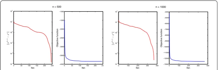
Figure 1Evolutions of the value ofxk+1–x∗and the objective function value with respect to the number of iterations forn= 500 andn= 1000
4 Numerical experiment
In this section, we apply the proposed method to solve a nonconvex optimization problem which arises in portfolio selection [25], neural network [26,27], and compressed sensing [28]. Some preliminary numerical results are reported to demonstrate the feasibility and advantage of the method. All numerical experiments are performed in MATLAB 2014b on a 64-bit PC with an Intel Core i7-7500U CPU (2.70 GHz) and 16 GB of RAM.
We consider the following optimization problem:
min1
2x
TAx–bTx+x 1
s.t.x∈S,
(21)
whereA∈Rn×nis a symmetric matrix that is not necessarily positive semidefinite,b∈Rn is a vector, S is a polyhedral set inRn. Problem (21) is obviously nonconvex. We also assume that the optimal value of (21) is finite and can be attained. Notice that one can write (21) equivalently as the following separable optimization problem:
minf(x) +g(x) (22)
by settingf(x) :=12xTAx–bTxandg(x) :=x
1+δ(x|S). In this setting,f is a possibly
non-convex function and∇f is Lipschitz continuous with modulusL> 0,gis a proper closed convex function, andf +gis level bounded. The parameterL=max{λmax(A),|λmin(A)|},
whereλmax(A) andλmin(A) are the largest and smallest eigenvalues ofArespectively.
Fur-thermore, the objective function in (21) satisfies the KL property as discussed in [14]. Therefore, we can apply the inexact proximal gradient algorithm with extrapolation in Algorithm (1) to solve the equivalent model (22).
In the numerical experiments, the test data of problem (21) is generated by the following way. We set the symmetric matrixA=D+DT∈Rn×n, whereDis a matrix generated with i.i.d. standard Gaussian entries; the polyhedral setS= [0, 1]n; the vectorbgenerated with i.i.d. standard Gaussian entries. We initialize thex0∈domg randomly and setx–1=x0.
Besides, the test method is terminated whenxk+1–xk ≤10–4and the maximal iteration
number is set as 5000.
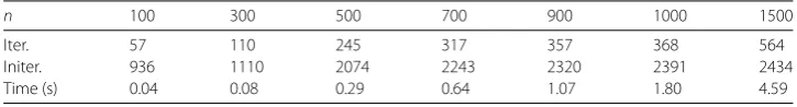
Table 1 Iteration number and CPU computing time of Algorithm1with different dimensions
n 100 300 500 700 900 1000 1500
Iter. 57 110 245 317 357 368 564
Initer. 936 1110 2074 2243 2320 2391 2434
Time (s) 0.04 0.08 0.29 0.64 1.07 1.80 4.59
{xk}is generated by the proposed inexact algorithm andx∗denotes the approximate so-lution obtained at termination of the algorithm. From Fig.1, we can see that the sequence xk+1–x∗converges to zero, and the objective function value decreases as the iteration
increases, which conforms with our theory. Furthermore, the number of iterations, inner iterations (the iteration needed to calculate the subproblem in the algorithm inexactly), and the cpu time (in seconds) required by the algorithm are reported in Table1for differ-ent dimensions of the problem, and are denoted as “Iter.”, “Initer.”, and “Time (s)” respec-tively. The results also indicate the feasibility and effectiveness of the proposed method.
5 Conclusions
In this paper, we proposed an inexact proximal gradient algorithm with extrapolation for solving a class of nonconvex optimization problems. The convergence of this inexact al-gorithm was established under the assumption that an auxiliary function satisfies the KL property. We proved that the iterative sequence generated by the proposed method con-verges to a stationary point of the problem. Furthermore, the convergence rate result was obtained by the means of KL exponent.
Funding
This work was supported by the National Natural Science Foundation of China (Grant No. 11801279), the Natural Science Foundation of Jiangsu Province (Grant No. BK20180782), and the Startup Foundation for Introducing Talent of NUIST (Grant No. 2017r059).
Competing interests
The authors declare that they have no competing interests.
Authors’ contributions
All authors contributed to drafting this manuscript. All authors read and approved the final manuscript.
Author details
1Department of Information and Computing Science, School of Mathematics and Statistics, Nanjing University of
Information Science and Technology, Nanjing, P.R. China. 2School of Economics and Management, Southeast University, Nanjing, P.R. China.3School of Mathematical Sciences, Nanjing Normal University, Nanjing, P.R. China.
Publisher’s Note
Springer Nature remains neutral with regard to jurisdictional claims in published maps and institutional affiliations.
Received: 15 March 2019 Accepted: 23 April 2019
References
1. Candès, E.J., Tao, T.: Decoding by linear programming. IEEE Trans. Inf. Theory51, 4203–4215 (2005) 2. Donoho, D.L.: Compressed sensing. IEEE Trans. Inf. Theory52, 1289–1306 (2006)
3. Chambolle, A.: An algorithm for total variation minimization and applications. J. Math. Imaging Vis.20, 89–97 (2004) 4. Bauschke, H.H., Combettes, P.L.: Convex Analysis and Monotone Operator Theory in Hilbert Spaces. Springer, New
York (2011)
5. Jia, Z.H., Cai, X.J.: A relaxation of the parameter in the forward-backward splitting method. Pac. J. Optim.13, 665–681 (2017)
6. O’Donoghue, B., Candès, E.J.: Adaptive restart for accelerated gradient schemes. Found. Comput. Math.15, 715–732 (2015)
8. Beck, A., Teboulle, M.: A fast iterative shrinkage-thresholding algorithm for linear inverse problems. SIAM J. Imaging Sci.2, 183–202 (2009)
9. Attouch, H., Bolte, J.: On the convergence of the proximal algorithm for nonsmooth functions involving analytic features. Math. Program.116, 5–16 (2009)
10. Attouch, H., Bolte, J., Redont, P., Soubeyran, A.: Proximal alternating minimization and projection methods for nonconvex problems: an approach based on the Kurdyka–Lojasiewicz inequality. Math. Oper. Res.35, 438–457 (2010) 11. Frankel, P., Garrigos, G., Peypouquet, J.: Splitting methods with variable metric for Kurdyka–Lojasiewicz functions and
general convergence rates. J. Optim. Theory Appl.165, 874–900 (2015)
12. Ochs, P., Chen, Y., Brox, T., Pock, T.: iPiano: inertial proximal algorithm for non-convex optimization. SIAM J. Imaging Sci.
7, 1388–1419 (2014)
13. Wen, B., Chen, X.J., Pong, T.K.: Linear convergence of proximal gradient algorithm with extrapolation for a class of nonconvex nonsmooth minimization problems. SIAM J. Optim.27, 124–145 (2017)
14. Attouch, H., Bolte, J., Svaiter, B.F., Soubeyran, A.: Convergence of descent methods for semi-algebraic and tame problems: proximal algorithms, forward-backward splitting, and regularized Gauss–Seidel methods. Math. Program.
137, 91–129 (2013)
15. Wu, Z.M., Li, M.: General inertial proximal gradient method for a class of nonconvex nonsmooth optimization problems. Comput. Optim. Appl. (2019).https://doi.org/10.1007/s10589-019-00073-1
16. Rockafellar, R.T.: Monotone operators and the proximal point algorithm. SIAM J. Control Optim.14, 877–898 (1976) 17. Solodov, M.V., Svaiter, B.F.: A hybrid approximate extragradient-proximal point algorithm using the enlargement of a
maximal monotone operator. Set-Valued Var. Anal.7, 323–345 (1999)
18. Solodov, M.V., Svaiter, B.F.: A hybrid projection-proximal point algorithm. J. Convex Anal.6, 59–70 (1999) 19. Solodov, M.V., Svaiter, B.F.: An inexact hybrid generalized proximal point algorithm and some new results on the
theory of Bregman functions. Math. Oper. Res.25, 214–230 (2000)
20. Li, G.Y., Pong, T.K.: Calculus of the exponent of Kurdyka–Łojasiewicz inequality and its applications to linear convergence of first-order methods. Found. Comput. Math.18, 1199–1232 (2018)
21. Bolte, J., Sabach, S., Teboulle, M.: Proximal alternating linearized minimization or nonconvex and nonsmooth problems. Math. Program.146, 459–494 (2014)
22. Nesterov, Y.: Introductory Lectures on Convex Optimization: A Basic Course. Kluwer Academic Publishers, Boston (2004)
23. Li, G.Y., Pong, T.K.: Douglas–Rachford splitting for nonconvex optimization with application to nonconvex feasibility problems. Math. Program.159, 371–401 (2016)
24. Xu, Y.Y., Yin, W.T.: A block coordinate descent method for regularized multi-convex optimization with applications to nonnegative tensor factorization and completion. SIAM J. Imaging Sci.6, 1758–1789 (2013)
25. Markowitz, H.: Portfolio selection. J. Finance7, 77–91 (1952)
26. Liu, Q.S., Dang, C.Y., Cao, J.D.: A novel recurrent neural network with one neuron and finite-time convergence for k-winners-take-all operation. IEEE Trans. Neural Netw.21, 1140–1148 (2010)
27. Liu, Q.S., Cao, J.D., Chen, G.R.: A novel recurrent neural network with finite-time convergence for linear programming. Neural Comput.22, 2962–2978 (2010)