A conjugate gradient algorithm and its application in large scale optimization problems and image restoration

(1)

R E S E A R C H

Open Access

A conjugate gradient algorithm and its

application in large-scale optimization

problems and image restoration

Gonglin Yuan

1

, Tingting Li

1

and Wujie Hu

1*

*_{Correspondence:}

[email protected] 1_{College of Mathematics and}

Information Science, Guangxi University, Nanning, P.R. China

Abstract

To solve large-scale unconstrained optimization problems, a modiﬁed PRP conjugate

gradient algorithm is proposed and is found to be interesting because it combines

the steepest descent algorithm with the conjugate gradient method and successfully

fully utilizes their excellent properties. For smooth functions, the objective algorithm

suﬃciently utilizes information about the gradient function and the previous

direction to determine the next search direction. For nonsmooth functions, a

Moreau–Yosida regularization is introduced into the proposed algorithm, which

simpliﬁes the process in addressing complex problems. The proposed algorithm has

the following characteristics: (i) a suﬃcient descent feature as well as a trust region

trait; (ii) the ability to achieve global convergence; (iii) numerical results for large-scale

smooth/nonsmooth functions prove that the proposed algorithm is outstanding

compared to other similar optimization methods; (iv) image restoration problems are

done to turn out that the given algorithm is successful.

MSC:

90C26

Keywords:

Conjugate gradient; Nonconvex and nonsmooth; Descent property;

Global convergence

1 Introduction

The concerned problem is given by

min

f

(

x

)

|

x

∈

n

,

(1.1)

where the function

f

:

n

→

and

f

∈

C

2

. The above model is quite typical but a

diﬃcult mathematic model and is seen throughout daily life, work, and scientiﬁc

re-search, thus being the focus of a great variety of careers. Experts and scholars have

conducted numerous in-depth studies and achieved a series of fruitful results (see, e.g.,

[

2

,

5

,

12

,

22

,

29

–

31

,

40

,

50

,

52

,

53

]). It is quite noticeable that the steepest descent method

is simple, and the computational and memory requirements are low. In the negative

gra-dient direction, the function’s value decreases rapidly, which makes it easy to think that

this is a suitable search direction, although the convergence rate of the gradient method

is not always fast. Later, experts and scholars modiﬁed this method and presented an

ef-ﬁcient conjugate gradient method, which provides a simple form but high performance.

(2)

There are two aspects of optimization problems: the step length and the search direction.

In general, the mathematical formula for (

1.1

) is

x

k+1

=

x

k

+

α

k

d

k

,

k

∈ {

0, 1, 2, . . .

}

,

(1.2)

where

x

k

is the current iteration point,

α

k

is called the step length, and

d

k

is the

k

th search

direction. The formula for

d

k

is often deﬁned by

d

k+1

=

⎧

⎨

⎩

–

g

k+1

+

β

k

d

k

,

if

k

≥

1,

–

g

k+1

,

if

k

= 0,

(1.3)

where

β

k

∈

. In addition, increasingly more eﬃcient and successful conjugate gradient

algorithms have been proposed using a variety of expression for

β

k

as well as

d

k

(see, e.g.,

[

9

,

11

,

27

,

38

,

42

–

44

,

47

,

49

]). The well-known PRP algorithm [

26

,

27

] is of the following

form:

β

_kPRP

=

g

T

k+1

(

g

k+1

–

g

k

)

g

(xk)2

,

(1.4)

where

g

k

,

g

k+1

and

f

k

denote

g

(

x

k

),

g

(

x

k+1

) and

f

(

x

k

), respectively.

g

(

x

k+1

) =

g

k+1

=

∇

f

(

x

k+1

)

is the gradient function of the objective function

f

at

x

k+1

. It is remarkable that the PRP

conjugate algorithm is extremely eﬀective for large-scale optimization problems. It is

re-grettable that it fails to achieve global convergence when addressing nonconvex function

problems under the so-called weak Wolfe–Powell (WWP) line search technique. Its

for-mula is as follows:

g

(

x

k

+

α

k

d

k

)

T

d

k

≥

ρ

g

kT

d

k

(1.5)

and

f

(

x

k

+

α

k

d

k

)

≤

f

k

+

ϕα

k

g

kT

d

k

,

(1.6)

where

ϕ

∈

(0, 1/2),

α

k

> 0 and

ρ

∈

(

ϕ

, 1). To address the above exchanging problem, Yuan,

Wei, and Lu [

48

] developed the following innovative formula for the normal WWP line

search technique (called Yuan, Wei, and Lu line search (YWL)) and obtained numerous

rich theoretical results:

f

(

x

k

+

α

k

d

k

)

≤

f

k

+

ϕα

k

g

kT

d

k

+

α

k

min

–

ϕ

1

g

kT

d

k

,

δ

α

k

2

d

k

2

(1.7)

and

g

(

x

k

+

α

k

d

k

)

T

d

k

≥

ρ

g

kT

d

k

+

min

–

ϕ

1

g

kT

d

k

,

δα

k

d

k

d

k

,

(1.8)

(3)

Armijo line search technique and proposed a modiﬁed Armijo line search technique as

follows:

f

(

x

k

+

α

k

d

k

)

≤

f

(

x

k

) +

λα

k

g

kT

d

k

+

α

k

min

–

λ

1

g

kT

d

k

,

λ

α

k

2

d

k

2

,

(1.9)

where

λ

,

γ

∈

(0, 1),

λ

1

∈

(0,

λ

), and

α

k

is the largest number of

{

γ

k

|

k

= 0, 1, 2, . . .

}

. It is

in-teresting that some scholars not only focus on the expression of the coeﬃcient

β

k

but also

attempt to modify the formula of the search direction

d

k+1

. Nonlinear conjugate

gradi-ent methods are increasingly more interesting to scholars because of their simplicity and

lower equipment requirements for the calculation environment. Thus, HS (see [

13

,

16

,

33

]) and PRP algorithms (see [

35

,

51

]) are widely used to solve complex problems in

vari-ous ﬁelds. Currently, some experts focus on the three-term conjugate gradient because its

search direction sometimes has the descent and automatic trust region properties.

Moti-vated by the above discussion, a new modiﬁed three-term conjugate gradient algorithm

based on the modiﬁed Armijo line search technique is proposed. The algorithm has the

following properties:

• The search direction has a suﬃcient decrease and a trust region property.

• For general functions, the proposed algorithm under mild assumptions possesses

global convergence.

• The new algorithm combines the deepest descent method with the conjugate gradient

algorithm through the size of the coeﬃcients, and the numerical results demonstrate

the method’s good performance compared with established algorithms.

• The corresponding numerical results prove that the discussed method is eﬃcient as

well as successful at solving general problems.

• The paper successfully combines the mathematic theory with real-world application.

On the one hand, the proposed algorithm has a good performance in solving the

large-scale optimization problems, on the other hand, it is introduced in the image

restoration, which has wild application in biological engineering, medical sciences

and other areas of science and engineering.

The remainder of this paper is organized as follows: The next section presents the

moti-vation and the content of the algorithm to solve large-scale smooth problems includes the

important mathematical characters; the similar optimization algorithm was presented to

solve large-scale non-smooth optimization problems; the Sect.

4

presents the application

of the Sect.

3

in the problem of the image restoration; the paper’s conclusion and

algo-rithm’s characters was listed in Sect.

5

. Without loss of generality,

f

(

x

k

) and

f

(

x

k+1

) are

replaced by

f

k

and

f

k+1

, and

·

is the Euclidean norm.

2 New three-term conjugate gradient algorithm for smooth problems

The three-term conjugate gradient algorithm has seen extensive study and obtained

ex-tremely good theoretical results. In the light of the work by Toouati-Ahmed, Storey [

34

],

Al-Baali [

1

], Gilbert, and Nocedal [

17

] on conjugate gradient methods, the suﬃcient

de-scent condition is crucial for the global convergence. From this, a famous formula for the

search direction

d

k+1

emerges. Zhang [

51

] proposed the following formula:

d

k+1

=

⎧

⎨

⎩

–

g

k+1

+

gT

k+1ykdk–dTkgk+1yk

gT

kgk

if

k

≥

1,

–

g

k+1

,

if

k

= 0,

(4)

where

y

k

=

g

k+1

–

g

k

. It is notable that the three-term conjugate gradient algorithm was

ﬁrstly introduced in solving optimization problems and the numeral results proves it is

competitive than similar methods, thus this paper choose it as the compared algorithm in

Sects.

2.3

and

3.2

. In [

23

], Nazareth proposed another variety of formula,

d

k+1

= –

y

k

+

y

T k

y

k

y

T_k

d

k

d

k

+

y

T k–1

y

k

y

T_k_–1

d

k–1

d

k–1

,

(2.2)

where

y

k

=

g

k+1

–

g

k

,

g

k

is the gradient function value at the point

x

k

, and

d

0

=

d

–1

= 0. In

[

14

], Deng and Zhong expressed a new three-term conjugate gradient formula as follows:

d

k+1

= –

g

k+1

–

1 –

y

T k

y

k

y

T k

s

k

s

T

k

g

k+1

y

T

k

s

k

–

y

T k

g

k+1

y

T

k

s

k

s

k

–

s

T k

g

k+1

y

T

k

s

k

y

k

,

(2.3)

where

s

k

=

x

k+1

–

x

k

. Based on the above discussion, we express the new three-term

algo-rithm under the modiﬁed Armijo line search technique (

1.9

) as follows:

d

k+1

=

⎧

⎨

⎩

–

g

k+1

+

gT_k₊₁y∗_kdk–dTkgk+1y∗k

max{ξ2dTky∗k,min(ξ3gk2,ξ4dTkdk)}

if

k

≥

1,

–

g

k+1

if

k

= 0,

(2.4)

where

ξ

2

,

ξ

3

,

ξ

4

> 0. To gather more information about the objective function, we address

the corresponding gradient function as well as the initial point, let

y

∗_k

=

y

k

+

ϕ

k

(

x

k+1

–

x

k

),

where

y

k

=

g

k+1

–

g

k

,

ϕ

k

=

max

{

0,

B

k

}

, and

B

k

=

(gk+1+gk)

T_s

k+2(fk–fk+1)

xk+1–xk2

. This plays an important

role in theory and numerical performance [

46

]. From the above discussion, we introduce

a new PRP algorithm (Algorithm

2.1

).

2.1 Algorithm steps

Algorithm 2.1

Step 1: (Initiation) Choose an initial point

x

0

,

γ

∈

(0, 1)

,

ξ

2

,

ξ

3

,

ξ

4

> 0

, and positive

con-stants

ε

∈

(0, 1)

. Let

k

= 0

,

d

0

= –

g

0

.

Step 2: If

g

k

≤

ε

, then stop.

Step 3: Find the step length, where the calculation

α

k

=

max

{

γ

k

|

k

= 0, 1, 2, . . .

}

stems

from (

1.9

).

Step 4: Set the new iteration point of

x

k+1

=

x

k

+

α

k

d

k

.

Step 5: Update the search direction by (

2.4

).

Step 6: If

g

k+1 ≤

ε

holds, the algorithm stops. Otherwise, go to next step.

Step 7: Let

k

:=

k

+ 1

and go to Step 3.

2.2 Algorithm characteristics

This section states the properties of the suﬃcient descent, trust region as well as global

convergence of Algorithm

2.1

.

Lemma 2.1

If the search direction d

k

is generated by

(

2.4

),

then

(5)

and

d

k

≤

(1 + 2/

ξ

2

)

g

k

,

(2.6)

where

σ

are positive constants

.

Proof

On the one hand, it is true that (

2.5

) and (

2.6

) are correct if

k

= 0.

On the other hand, from (

2.4

),

g

_kT₊₁

d

k+1

=

g

kT+1

–

g

k+1

+

g

T

k+1

y

∗k

d

k

–

d

Tk

g

k+1

y

∗k

max

{

ξ

2

d

_kT

y

∗_k

,

min(

ξ

3

g

k

2

,

ξ

4

d

kT

d

k

)

}

= –

g

k+12

+

g

_kT₊₁

g

_kT₊₁

y

∗_k

d

k

–

g

kT+1

d

Tk

g

k+1

y

∗k

max

{

ξ

2

d

T

k

y

∗k

,

min(

ξ

3

g

k

2

,

ξ

4

d

Tk

d

k

)

}

= –

g

k+12

and

d

k+1

=

g

k+1

+

g

T

k+1

y

∗k

d

k

–

d

Tk

g

k+1

y

∗k

max

{

ξ

2

d

_kT

y

∗_k

,

min(

ξ

3

g

k

2

,

ξ

4

d

Tk

d

k

)

}

≤

g

k+1

+

g

kT+1

y

∗k

d

k

–

d

kT

g

k+1

y

∗k

max

{

ξ

2

d

T

k

y

∗k

,

min(

ξ

3

g

k

2

,

ξ

4

d

kT

d

k

)

}

≤

g

k+1

+

g

k+1

y

∗k

d

k

+

d

k

g

k+1

y

∗k

ξ

2

d

T k

y

∗k

≤

g

k+1

+ 2

g

k+1

y

∗k

d

k

ξ

2

d

T k

y

∗k

= (1 + 2/

ξ

2

)

g

k+1

.

(2.7)

It is true that (

2.5

) and (

2.6

) demonstrate that the search direction has a suﬃcient descent

trait and a trust region property, respectively.

Aiming at achieving global convergence, we propose the following mild assumptions.

Assumption (i)

The level set of

Ω

=

{

x

|

f

(

x

)

≤

f

(

x

0

)

}

is bounded.

Assumption (ii)

The objective function

f

(

x

)

∈

C

2

is bounded from below, and its gradient

function

g

(

x

) is Lipschitz continuous, i.e., there exists a positive constant

τ

such that

g

(

x

) –

g

(

y

)

≤

τ

x

–

y

,

x

,

y

∈

R

n

.

(2.8)

Based on the above discussion and established conclusion concerning the modiﬁed

Armijo line search of being reasonable and necessary (see [

48

]), the global convergence

algorithm is established as follows.

Theorem 2.1

If assumptions

(i)

–

(ii)

are true and the corresponding sequences of

{

x

k

}

,

{

d

k

}

,

{

g

k

}

,

{

α

k

}

are generated by Algorithm

2.1

,

then we arrive at the conclusion that

lim

(6)

Proof

Suppose that the conclusion of the above theorem is incorrect, i.e., there exist a

positive constant

σ

3

and index number

k

such that

g

k

≥

σ

3

,

∀

k

≥

k

.

(2.10)

Based on (

1.9

) and (

2.5

),

f

(

x

k

+

α

k

d

k

)

≤

f

(

x

k

) +

λα

k

g

Tk

d

k

+

α

k

min

–

λ

1

g

kT

d

k

,

λ

α

k

2

d

k

2

≤

f

(

x

k

) +

α

k

(

λ

–

λ

1

)

g

Tk

d

k

.

Then with the above formulas with

k

= 0 from

∞

and combining with Assumption

(ii)

, we

obtain

∞

k=0

α

k

(

λ

–

λ

1

)

g

Tk

d

k

≤

f

0

–

f

∞

<

∞

.

(2.11)

Based on the convergence theorem of sequences,

lim

k→∞

(

λ

–

λ

1

)

α

k

g

T

k

d

k

= 0.

(2.12)

Then we have

lim

k→∞

α

k

g

T

k

d

k

= 0,

(2.13)

from the formula of (

2.5

), then

lim

k→∞

α

k

g

k

2

= 0.

(2.14)

This means that

{

α

k

} →

0,

k

→ ∞

or

{

g

k

} →

0,

k

→ ∞

. We then state two cases:

(i) If

{

α

k

} →

0,

k

→ ∞

, consider the line search method, for every suitable parameter

α

k

,

f

(

x

k

+

α

k

/

γ

d

k

) >

f

(

x

k

) +

λα

k

/

γ

g

Tk

d

k

+

α

k

/

γ

min

–

λ

1

g

kT

d

k

,

λα

k

d

k

2

/(2

γ

)

,

there thus exists a positive constant

λ

∗

≤

λ

1

, such that

f

(

x

k

+

α

k

d

k

/

γ

) –

f

(

x

k

)

≥

–

λ

–

λ

∗

α

k

/

γ

g

k

2

.

Using (

2.5

), Assumption

(ii)

and the continuity of

f

(

x

) and

g

(

x

), we have

f

(

x

k

+

α

k

d

k

/

γ

) –

f

(

x

k

) =

α

k

/

γ

g

(

x

k

+

η

k

α

k

/

γ

d

k

)

T

d

k

=

α

k

/

γ

g

(

x

k

)

T

d

k

+

α

k

/

γ

g

(

x

k

+

η

k

α

k

/

γ

d

k

) –

g

(

x

k

)

T

d

k

≤

α

k

/

γ

g

(

x

k

)

T

d

k

+

η

k

τ α

k2

/

γ

2

d

k

2

= –

α

k

/

γ

g

(

x

k

)

2

(7)

where

η

k

∈

(0, 1). Comparing the above two expressions, we have

–

α

k

/

γ

g

xk

2

+

η

k

τ α

2k

/

γ

2

d

k

2

≥

–

λ

–

λ

∗

/

γ α

k

g

xk

2

i.e.,

g

xk

2

–

η

k

τ α

k

/

γ

d

k2

≤

λ

–

λ

∗

g

(

x

k

)

2

.

Thus,

α

k

≥

γ

1 –

λ

+

λ

∗

/

η

k

τ σ

2

> 0,

where

σ

∈

(1 +

2

ξ2

,

∞

). This contradicts the assumption of case (i).

(ii) Clearly,

{

g

k

} →

0 if

α

k

is a positive ﬁnite constant when

k

is a suﬃciently large

con-stant from the formula of (

2.14

). This conclusion does not satisfy the assumption of (

2.10

);

this completes the proof.

2.3 Numerical results

Related content is presented in this section and consists of two parts: test problems and

corresponding numerical results. To measure the algorithm’s eﬃciency, we compare

Al-gorithm

2.1

with Algorithm 1 in [

51

] in terms of NI, NFG, and CPU on the test problems

listed in Table

2

of Appendix

1

, which are from [

3

], where NI, NFG, and CPU indicate

the number of iterations, the sum of the calculation’s frequency of the objective function

and gradient function, and the calculation time needed to solve various test problems (in

seconds), respectively. Algorithm 1 is diﬀerent from the objective algorithm in the

for-mula of

d

k+1

that was determined by (

2.1

), and the remainder of Algorithm 1 is identical

to Algorithm

2.1

.

Stopping rule

: If

|

f

(

x

k

)

|

>

e

1

, let

stop

1 =

|f(xk_|)–_f₍_xf_k(x_)|k+1)|

or

stop

1 =

|

f

(

x

k

) –

f

(

x

k+1

)

|

. If the

condition

g

(

x

)

<

or

stop

1 <

e

2

is satisﬁed, the algorithm stops, where

e

1

=

e

2

= 10

–4

,

= 10

–4

. On the one hand, based on the virtual case, the proposed algorithm also stops if

the number of iterations is greater than 10,000 and the iteration number of

α

k

is greater

than 5. On the other hand, ‘NO’ and ‘problem’ in Table

2

indicate the number of the tested

problem and the name of the problem, respectively.

Initiation

:

λ

= 0.9,

λ

1

= 0.4,

ξ

3

= 300,

ξ

2

=

ξ

4

= 0.01,

γ

= 0.01.

Dimension

: 30,000, 90,000, 150,000, 210,000.

Calculation environment

: The calculation environment is a computer with 2 GB of

memory, a Pentium (R) Dual-Core CPU [email protected] GHz, and the 64-bit Windows 7

op-erating system.

(8)

[image:8.595.115.480.79.501.2]

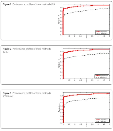
Figure 1Performance proﬁles of these methods (NI)

Figure 2Performance proﬁles of these methods (NFG)

Figure 3Performance proﬁles of these methods (CPU time)

red curve’s value of the initial point is close to 0.9, while Algorithm 1 only arrives at a

value of 0.6. This means that Algorithm

2.1

addresses complex problems fewer iterations.

In Fig.

2

, the red curve is above the left curve because the calculation number of the

ob-jective function is less than the left one when addressing practical problems, which is an

important aspect for measuring the performance of an algorithm. It is well know that the

calculation time (CPU time) is the most essential metric of an algorithm because the speed

of the algorithm is the most basic feature. The objective algorithm not only is well deﬁned

because the curve seems more feasible and smooth but also can address most complex

problems because the largest value of the point on the curve is close to 0.98, which

in-dicates that the proposed algorithm is highly eﬀective. Overall, the proposed algorithm

cannot only solve smooth problems but it also enriches the knowledge of optimization

and lays the foundation for further in-depth studies.

3 Algorithm for nonsmooth problems

(9)

pro-posed method to nonsmooth problems. It is interesting that the vast majority of practical

conditions are harsh; therefore, Newton’s series of methods are often unsatisfactory for

solving such problems because they require information about the gradient function [

37

,

39

,

46

]. Currently, most experts and scholars focus on bundled methods, which are

suc-cessful solutions to small-scale problems (see [

18

,

19

,

24

,

36

]) but fail to solve large-scale

practical problems. With the development of science and technology, it is becoming an

ur-gent need to design a simple but eﬀective algorithm to solve large-scale nonsmooth

prob-lems. Based on the simplicity of the conjugate gradient method, some experts and scholars

have proposed relevant algorithms and made numerous fruitful theoretical achievements

(see [

20

,

28

]).

Consider the following problem:

min

θ

(

x

),

(3.1)

where

θ

(

x

) sometimes is nonsmooth and

x

∈

R

n

. A famous technique is called ‘Moreau–

Yosida’ regularization, which calculates the equivalent solution of the previous problem

through a modiﬁed object function with the formula

min

t∈Rn

θ

(

t

) +

t

–

x

2

χ

,

(3.2)

where

χ

and

·

denote a positive constant and the Euclidean norm, respectively. Without

loss of generality, we denote

θ

M

(

x

) as in (

3.1

) ‘Moreau–Yosida’ regularization, i.e.,

θ

M

(

x

) =

min

t∈Rn

θ

(

t

) +

t

–

x

2

χ

.

(3.3)

The ‘Moreau–Yosida’ regularization technique was introduced because of its

outstand-ing properties such as diﬀerentiability (see [

21

,

25

]). Assume that the function (

3.1

) is

convex and that its ‘Moreau–Yosida’ regularization obtains the best solution of

ω

(

x

) =

argmin

θ

M

(

t

). Based on the mathematic knowledge and the established conclusion, we

then have

∇

θ

M

(

x

) =

ω

(

x

) –

x

χ

.

(3.4)

(10)

3.1 New algorithm and its necessary properties

We start with the following formula for

d

k+1

, which is an important component of the

proposed algorithm in addressing complex problems:

d

k+1

=

⎧

⎨

⎩

–

∇

θ

M

(

x

k+1

)

T

+

∇θM(xk+1)ykdk–dTk∇θM(xk+1)yk

max{ξ2dkyk,min{ξ3∇θM(xk)2,ξ4dk2}}

,

if

k

≥

1,

–

∇

θ

M

(

x

k+1

),

if

k

= 0,

(3.5)

where

s

k

=

x

k+1

–

x

k

,

y

k

=

∇

θ

M

(

x

k+1

) –

∇

θ

M

(

x

k

), and

ξ

2

,

ξ

3

, and

ξ

4

are positive constants.

The step length

α

k

is determined by

θ

M

(

x

k

+

α

k

d

k

)

≤

θ

M

(

x

k

) +

λα

k

∇

θ

M

(

x

k

)

T

d

k

+

α

k

min

–

λ

1∇

θ

M

(

x

k

)

T

d

k

,

λα

k

d

kT

d

k

/2

,

(3.6)

where

λ

,

γ

∈

(0, 1),

λ

1

∈

(0,

λ

), and

α

k

is the largest number of

{

γ

k

|

k

= 0, 1, 2, . . .

}

. It is

well known from the case of smooth functions that the new search direction has

satisfac-tory descent and trust region properties; therefore, we merely list them without proof. We

have

∇

θ

M

(

x

k

)

T

d

k

= –

∇

θ

M

(

x

k

)

2

,

(3.7)

d

k

≤

σ

∇

θ

M

(

x

k

)

,

(3.8)

where

σ

is the same as in (

2.7

). Now, manifesting speciﬁc algorithm steps, we

ex-press the cause of the existing

α

_k

∈

that satisﬁes the demands of the modiﬁed

Armijo line search formula and provides the global convergence of the proposed

algo-rithm.

Algorithm 3.1

Step 1: (Initiation) Choose an initial point

x

0

,

γ

∈

(0, 1)

,

ξ

2

,

ξ

3

, and

ξ

4

> 0

and positive

constants

ε

∈

(0, 1)

. Let

k

= 0

,

d

0

= –

∇

θ

M

(

x

0

)

.

Step 2: If

∇

θ

M

(

x

k

)

≤

ε

, then stop.

Step 3: Find the step length, i.e., the calculation

α

k

=

max

{

γ

k

|

k

= 0, 1, 2, . . .

}

stemming

from (

3.6

).

Step 4: Set the new iteration point

x

k+1

=

x

k

+

α

k

d

k

.

Step 5: Update the search direction by (

3.5

).

Step 6: If

∇

θ

M

(

x

k+1

)

≤

ε

holds, the algorithm stops; otherwise, go to the next step.

Step 7: Let

k

:=

k

+ 1

and go to Step 3.

To express the validity of the step length

α

k

in (

3.6

) and the global convergence of

Algo-rithm

3.1

, the following assumptions are necessary.

Assumption

(i) The level set

π

=

{

x

|

θ

M

(

x

)

≤

θ

M

(

x

0

)

}

is bounded.

(11)

From the ‘Moreau–Yosida’ regularization technique, the function

θ

M

(

x

) is Lipschitz

con-tinuous, i.e., there exists a positive constant

κ

subject to

∇

θ

M

(

x

) –

∇

θ

M

(

y

)

≤

κ

x

–

y

.

(3.9)

Theorem 3.1

If Assumptions

(i)

–

(ii)

are true

,

then there exists a constant

α

k

that satisﬁes

the requirements of

(

3.6

).

Proof

We introduce the following function:

ϑ

(

α

) =

θ

M

(

x

k

+

α

d

k

) –

θ

M

(

x

k

) –

λα

∇

θ

M

(

x

k

)

T

d

k

–

α

min

–

λ

1∇

θ

M

(

x

k

)

d

k

,

λα

d

Tk

d

k

/2

.

(3.10)

Based on the established theorem, following the suﬃcient decrease of (

3.7

), for suﬃciently

small positive

α

, we have

ϑ

(

α

) =

θ

M

(

x

k

+

α

d

k

) –

θ

M

(

x

k

) –

λα

∇

θ

M

(

x

k

)

T

d

k

–

α

min

–

λ

1∇

θ

M

(

x

k

)

T

d

k

,

λα

d

Tk

d

k

/2

=

α

(1 +

λ

1

–

λ

)

∇

θ

M

(

x

k

)

T

d

k

+

o

(

α

) < 0,

where the latter inequality holds since the objective function is continuous. Thus, there

exists a constant 0 <

α

0

< 1 such that

ϑ

(

α

0

) < 0; on the other hand,

ϑ

(0) = 0, and based on

the function’s continuous property, there exists a constant

α

1

such that

ϑ

(

α

1

) =

θ

M

(

x

k

+

α

1

d

k

) –

θ

M

(

x

k

) –

λα

1∇

θ

M

(

x

k

)

T

d

k

–

α

1

min

–

λ

1∇

θ

M

(

x

k

)

d

k

,

λα

1

d

Tk

d

k

/2

< 0.

Thus,

θ

M

(

x

k

+

α

1

d

k

) <

θ

M

(

x

k

) +

λα

1∇

θ

M

(

x

k

)

T

d

k

+

α

1

min

–

λ

1∇

θ

M

(

x

k

)

T

d

k

,

λα

1

d

Tk

d

k

/2

is correct, and this means that the modiﬁed Armijo line search is well deﬁned. From the

above discussion, Algorithm

3.1

has the properties of the suﬃcient descent and a trust

region, and we can now present the theorem of global convergence.

Theorem 3.2

If the above assumptions are satisﬁed and the relative sequences

{

x

k

}

,

{

α

k

}

,

{

d

k

}

,

{

θ

M

(

x

k

)

}

are generated by Algorithm

3.1

,

then we have

lim

k→∞

∇

θ

M

(

x

k

)

= 0.

We neglect the proof because its proof is similar to that of Theorem

2.1

.

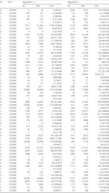
3.2 Nonsmooth numerical experiment

(12)

addition, the problems are only diﬀerent from Algorithm

3.1

in the formula for

d

k+1

. The

relevant numerical data are listed in Table

5

of Appendix

2

, and we plot the corresponding

graphs based on these data, where ‘NI’, ‘NF’, and ‘CPU’ are the iteration number,

calcula-tion number of the objective funccalcula-tion and the algorithm’s run time (in seconds). The ﬁrst

metric is determined by

d

k+1

=

⎧

⎨

⎩

–

∇

θ

M

(

x

k+1

) +

∇

θM(xk+1))Tykdk–dTk∇θM(xk+1)yk ∇θM₍_x

k)T∇θM(xk)

,

if

k

≥

1,

–

∇

θ

M

(

x

k+1

),

if

k

= 0.

(3.11)

In [

51

], without loss of generality, calling Algorithm 2, the other algorithm in [

4

] is

calcu-lated as

d

k+1

=

⎧

⎨

⎩

–yT_ksk∇θM(xk+1)+yTk∇θM(xk+1)sk–sTkgk+1yk ∇θM₍_x

k)2

,

if

k

≥

1,

–

∇

θ

M

(

x

k+1

),

if

k

= 0,

(3.12)

denoted as Algorithm 3.

Dimension

: 150,000, 180,000, 192,000, 210,000, 222,000, 231,000, 240,000, 252,000,

270,000.

Initiation

:

λ

= 0.9,

λ

1

= 0.4,

ξ

3

= 100,

ξ

2

=

ξ

4

= 0.01,

γ

= 0.5.

Stopping rule

: If NI is no greater than 10,000,

|

f

(

x

k+1

) –

f

(

x

k

)

|

< 1

e

– 7 and if the iteration

number of

α

k

is no greater than 5, then the algorithm stops.

Calculation environment

: The calculation environment is a computer with 2 GB of

memory, a Pentium (R) Dual-Core CPU [email protected] GHz and the 64-bit Windows 7

op-erating system.

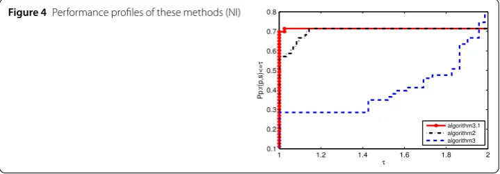
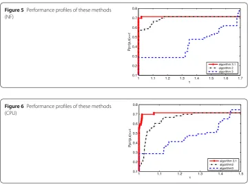
From Figs.

4

–

6

, the proposed algorithm is eﬀective and successful to a large extent. First,

the computational data of the algorithm fully address complex situations. Second, the

al-gorithm in the design of the search direction carefully considers the corresponding

func-tion, gradient function and current direction. In Figs.

4

and

5

, the curve of Algorithm

3.1

[image:12.595.118.478.609.734.2]

is above the other two curves because the number of iterations is much lower. Its initial

point is close to 0.75, which is much larger than the other algorithms. Note that the

pro-posed algorithm’s computation time is the best of the three algorithms because the curve

increases rapidly and is very smooth. In other words, its curve has a wonderful initiation

point, which results in a high eﬃciency in addressing complex issues.

(13)

[image:13.595.117.478.79.348.2]

Figure 5Performance proﬁles of these methods (NF)

Figure 6Performance proﬁles of these methods (CPU)

4 Applications of Algorithm

3.1

in image restoration

It is well known that many modern applications of optimization call for studying

large-scale nonsmooth convex optimization problems, where the image restoration problem

arising in image processing is an illustrating example. The image restoration problem plays

an important role in biological engineering, medical sciences and other areas of science

and engineering (see [

6

,

10

,

32

] etc.), which is to reconstruct an image of an unknown

scene from an observed image. The most common image degradation model is deﬁned by

the following system:

b

=

Ax

+

η

,

where

x

∈

n

is the underlying images,

b

∈

m

is the observed images,

A

is an

m

×

n

blurring matrix, and

η

∈

m

denotes the noise. One way to get the unknown

η

is to solving

the problem

min

x∈n

Ax

+

b

2

. This problem will not have a satisfactory solution since the

system is very sensitive to lack of information and the noise. The regularized least square

problem is often used to overcome the above shortcoming

min

x∈n

Ax

+

b

2

+

λ

Dx

1

,

where

· 1

is the

l

1

norm,

λ

is the regularization parameter controlling the trade-oﬀ

between the regularization term and the data-ﬁtting term, and

D

is a linear operator. It is

easy to see that the above problem is a nonsmooth convex optimization problem and it is

typically of large scale since the

l

1

norm is nonsmooth.

4.1 Image restoration problem

(14)

[image:14.595.118.410.270.427.2]

Table 1

The CPU time of PRP algorithm and Algorithm

3.1

in seconds

Lena Cameraman Barbara Banoon Man

20% noise

PRP algorithm 1.796875 9.6875 1.421875 1.375 3.375

Algorithm3.1 1.375 0.765625 1.46875 1.40625 3.328125

50% noise

PRP algorithm 1.98437 1.000 2.296875 1.71875 5.1875

Algorithm3.1 1.82812 0.921875 1.96875 1.8125 4.953125

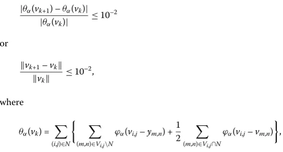
parameters are the same as those of Sect.

3.2

diﬀerent from

ξ

2

=

ξ

3

=

ξ

4

= 1. All codes are

written by MATLAB r2017a and run on a PC with an Intel Pentium(R) Xeon(R) E5507

CPU @2.27 GHz, 6.00 GB of RAM, and the Windows 7 operating system. The stopped

condition is

|

θ

α

(

v

k+1

) –

θ

α

(

v

k

)

|

θ

α

(

v

k

)

|

≤

10

–2

or

v

k+1

–

v

k

v

k

≤

10

–2

,

where

θ

α

(

v

k

) =

(i,j)∈N (m,n)∈Vi,j\N

ϕ

α

(

v

i,j

–

y

m,n

) +

1

2

(m,n)∈Vi,j∩N

ϕ

α

(

v

i,j

–

v

m,n

)

,

the noise candidate indices set

N

:=

{

(

i

,

j

)

∈

A

| ¯

y

i,j

=

y

i,j

,

y

i,j

=

s

min

or

s

max}

,

s

max

is the

maxi-mum of the noisy pixel and

s

min

denotes the minimum of the noisy pixel,

A

=

{

1, 2, . . . ,

M

}×

{

1, 2, 3, . . . ,

N

}

,

V

i,j

=

{

(

i

,

j

– 1), (

i

,

j

+ 1), (

i

– 1,

j

), (

i

+ 1,

j

)

}

is the neighborhood of (

i

,

j

),

y

de-notes the observed noisy image of

x

corrupted by the salt-and-pepper noise,

y

¯

is deﬁned

by the image obtained by applying the adaptive median ﬁlter method to the noisy image

y

in the ﬁrst phase,

x

is the true image with

M

-by-

N

pixels, and

x

i,j

denotes the gray level

of

x

at pixel location (

i

,

j

). It is easy to see that the regularity of

θ

α

only depends on

ϕ

α

and there exist many properties as regards

θ

α

and

ϕ

α

that are studied by many scholars

(see [

7

,

8

] etc.). In the experiments, Lena (256

×

256), Cameraman (256

×

256), Barbara

(512

×

512), Banoon (512

×

512), and Man (1024

×

1024) are the tested images. To

com-pare Algorithm

3.1

with other similar algorithm, we also test the well-known PRP

conju-gate gradient algorithm, where the Step 5 of Algorithm

3.1

is replaced by the PRP formula.

The tested performances of these two algorithms (Algorithm

3.1

and PRP algorithm) are

listed and the spent time is stated in Table

1

.

4.2 Results and discussion

(15)

[image:15.595.117.477.79.577.2]

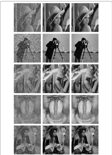
Figure 7Restoration of the images Lena, Cameraman, Barbara, Banoon, and Man by PRP algorithm and Algorithm3.1. From left to right: the noisy image with 20% salt-and-pepper noise, the restorations obtained by minimizingzwith PRP algorithm and Algorithm3.1, respectively

5 Conclusion

(16)

[image:16.595.117.477.79.577.2]

Figure 8Restoration of the images Lena, Cameraman, Barbara, Banoon, and Man by PRP algorithm and Algorithm3.1. From left to right: the noisy image with 50% salt-and-pepper noise, the restorations obtained by minimizingzwith PRP algorithm and Algorithm3.1, respectively

(17)

[image:17.595.119.475.132.477.2]

Appendix 1

Table 2

Test problems

No. Problem

1 Extended Freudenstein and Roth Function 2 Extended Trigonometric Function

3 Extended Rosenbrock Function

4 Extended White and Holst Function

5 Extended Beale Function

6 Raydan 1 Function

7 Raydan 2 Function

8 Diagonal 1 Function

10 Hager Function

11 Generalized Tridiagonal 1 Function 12 Extended Tridiagonal 1 Function

13 Extended Three Exponential Terms Function 14 Generalized Tridiagonal 2 Function

17 Extended Himmelblau Function 18 Generalized PSC1 Function

19 Extended PSC1 Function

20 Extended Powell Function

21 Extended Block Diagonal BD1 Function 22 Extended Maratos Function

23 Extended Cliﬀ Function

24 Quadratic Diagonal Perturbed Function

25 Extended Wood Function

26 Extended Hiebert Function 27 Quadratic Function QF1 Function 28 Extended Quadratic Penalty QP1 Function 29 Extended Quadratic Penalty QP2 Function 30 A Quadratic Function QF2 Function

31 Extended EP1 Function

32 BDQRTIC (CUTE)

No. Problem

33 TRIDIA Function (CUTE)

34 ARWHEAD Function (CUTE)

35 NONDQUAR Function (CUTE)

36 DQDRTIC Function (CUTE)

37 EG2 Function (CUTE)

38 DIXMAANA Function (CUTE)

39 DIXMAANB Function (CUTE)

40 DIXMAANC Function (CUTE)

41 DIXMAANE Function (CUTE)

42 Broyden Tridiagonal Function 43 Almost Perturbed Quadratic Function 44 Tridiagonal Perturbed Quadratic Function

45 EDENSCH Function (CUTE)

46 STAIRCASE S1 Function

47 LIARWHD Function (CUTE)

48 DIAGONAL 6 Function

49 DIXON3DQ Function (CUTE)

50 DIXMAANF Function (CUTE)

51 DIXMAANG Function (CUTE)

52 DIXMAANH Function (CUTE)

53 DIXMAANJ Function (CUTE)

54 DIXMAANL Function (CUTE)

55 DIXMAAND Function (CUTE)

56 ENGVAL1 Function (CUTE)

57 FLETCHCR Function (CUTE)

58 COSINE Function (CUTE)

59 Extended DENSCHNB Function (CUTE)

60 DENSCHNF Function (CUTE)

61 SINQUAD Function (CUTE)

62 BIGGSB1 Function (CUTE)

63 Partial Perturbed Quadratic PPQ2 Function 64 Scaled Quadratic SQ1 Function

65 BDQRTIC Function (CUTE)

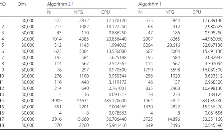
Table 3

Numerical results

NO Dim Algorithm2.1 Algorithm 1

NI NFG CPU NI NFG CPU

1 30,000 572 2832 17.170120 575 2844 17.689130

2 30,000 217 1082 10.122250 63 312 2.980625

3 30,000 43 170 0.886250 47 186 0.995250

4 30,000 1014 4385 23.856440 2007 8265 44.962060

5 30,000 312 1145 1.994063 5204 20,616 32.667130

6 30,000 623 3084 13.556880 607 3004 15.491130

7 30,000 195 584 1.625188 195 584 2.082937

8 30,000 114 567 2.542562 114 567 3.302094

9 30,000 78 297 0.970500 1799 3598 16.080500

10 30,000 276 1100 3.950344 256 1020 3.633312

11 30,000 116 448 3.119172 46 137 0.968500

12 30,000 214 640 2.761031 835 2460 10.498130

13 30,000 5 16 0.093313 78 233 1.184125

14 30,000 4909 19,634 285.120600 1464 5821 83.039530

15 30,000 551 2201 7.004469 1430 4822 15.256470

16 30,000 4 8 0.078563 4 8 0.061656

17 30,000 3916 15,660 56.706440 3725 14,896 53.351160

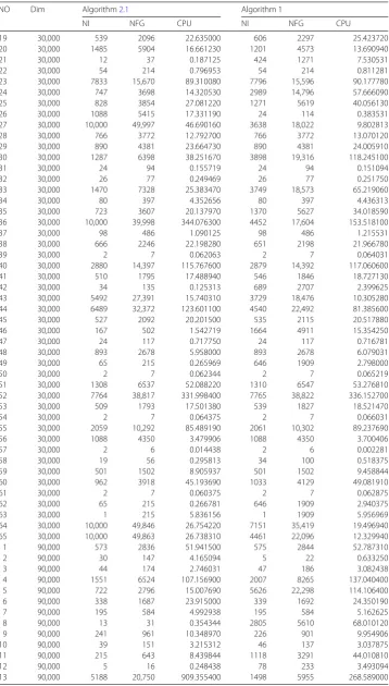
[image:17.595.119.478.522.732.2]

(18)

[image:18.595.119.478.98.729.2]

Table 3

(

Continued

)

NI NFG CPU NI NFG CPU

19 30,000 539 2096 22.635000 606 2297 25.423720

20 30,000 1485 5904 16.661230 1201 4573 13.690940

21 30,000 12 37 0.187125 424 1271 7.530531

22 30,000 54 214 0.796953 54 214 0.811281

23 30,000 7833 15,670 89.310080 7796 15,596 90.177780

24 30,000 747 3698 14.320530 2989 14,796 57.666090

25 30,000 828 3854 27.081220 1271 5619 40.056130

26 30,000 1088 5415 17.331190 24 114 0.383531

27 30,000 10,000 49,997 46.690160 3638 18,022 9.802813

28 30,000 766 3772 12.792700 766 3772 13.070120

29 30,000 890 4381 23.664730 890 4381 24.005910

30 30,000 1287 6398 38.251670 3898 19,316 118.245100

31 30,000 24 94 0.155719 24 94 0.151094

32 30,000 26 77 0.249469 26 77 0.251750

33 30,000 1470 7328 25.383470 3749 18,573 65.219060

34 30,000 80 397 4.352656 80 397 4.436313

35 30,000 723 3607 20.137970 1370 5627 34.018590

36 30,000 10,000 39,998 344.076300 4452 17,604 153.518100

37 30,000 98 486 1.090125 98 486 1.215531

38 30,000 666 2246 22.198280 651 2198 21.966780

39 30,000 2 7 0.062063 2 7 0.064031

40 30,000 2880 14,397 115.767600 2879 14,392 117.060600

41 30,000 510 1795 17.488940 546 1846 18.727130

42 30,000 34 135 0.125313 689 2707 2.399625

43 30,000 5492 27,391 15.740310 3729 18,476 10.305280

44 30,000 6489 32,372 123.601100 4540 22,492 81.385600

45 30,000 527 2092 20.201500 535 2115 20.517880

46 30,000 167 502 1.542719 1664 4911 15.354250

47 30,000 24 117 0.717750 24 117 0.716781

48 30,000 893 2678 5.958000 893 2678 6.079031

49 30,000 65 215 0.265969 646 1909 2.798000

50 30,000 2 7 0.062344 2 7 0.065219

51 30,000 1308 6537 52.088220 1310 6547 53.276810

52 30,000 7764 38,817 331.998400 7765 38,822 336.152700

53 30,000 509 1793 17.501380 539 1827 18.521470

54 30,000 2 7 0.064375 2 7 0.066031

55 30,000 2059 10,292 85.489190 2061 10,302 89.237690

56 30,000 1088 4350 3.479906 1088 4350 3.700406

57 30,000 2 6 0.014438 2 6 0.002281

58 30,000 19 56 0.295813 34 100 0.518375

59 30,000 501 1502 8.905937 501 1502 9.458844

60 30,000 962 3918 45.193690 1033 4129 49.081910

61 30,000 2 7 0.060375 2 7 0.062875

62 30,000 65 215 0.266781 646 1909 2.940375

63 30,000 1 215 5.836156 1 1909 5.956969

64 30,000 10,000 49,846 26.754220 7151 35,419 19.496940

65 30,000 10,000 49,863 26.738310 4461 22,096 12.329940

1 90,000 573 2836 51.941500 575 2844 52.787310

2 90,000 30 147 4.165094 5 22 0.633250

3 90,000 44 174 2.746031 47 186 3.082438

4 90,000 1551 6524 107.156900 2007 8265 137.040400

5 90,000 722 2796 15.007690 5626 22,298 114.106400

6 90,000 338 1687 23.915000 339 1692 24.350190

7 90,000 195 584 4.992938 195 584 5.162625

8 90,000 13 31 0.354344 2805 5610 68.010120

9 90,000 241 961 10.348970 226 901 9.954906

10 90,000 39 151 3.215312 46 137 3.037875

11 90,000 215 643 8.439844 1118 3291 44.010810

12 90,000 5 16 0.248438 78 233 3.493094

(19)

[image:19.595.122.476.100.729.2]

Table 3

(

Continued

)

NI NFG CPU NI NFG CPU

14 90,000 854 3388 33.367970 1485 4987 50.862160

15 90,000 4 8 0.203781 4 8 0.201875

16 90,000 4097 16,384 181.834700 3938 15,748 178.470700

17 90,000 577 2282 139.602700 651 2501 151.183100

18 90,000 540 2099 68.454150 606 2297 76.485500

19 90,000 1912 7602 66.348030 1201 4573 42.566220

20 90,000 35 108 1.810375 450 1349 24.126810

21 90,000 54 214 2.466781 54 214 2.486906

22 90,000 7833 15,670 274.592900 7796 15,596 283.996600

23 90,000 93 460 5.444188 1085 5312 66.299620

24 90,000 961 4387 93.333880 1271 5619 120.455800

25 90,000 1088 5415 53.056840 24 114 1.183812

26 90,000 2051 10180 20.263250 3731 18,486 35.322310

27 90,000 748 3701 38.751530 748 3701 39.540090

28 90,000 891 4387 71.637530 891 4387 72.518130

29 90,000 1284 6402 105.456800 3898 19,320 332.476700

30 90,000 24 94 0.467781 24 94 0.483219

31 90,000 26 77 0.779031 26 77 0.777844

32 90,000 1133 5635 59.076220 3249 16,242 190.573400

33 90,000 24 117 3.867094 24 117 3.884219

34 90,000 714 3565 60.103160 1650 7029 125.869400

35 90,000 10,000 39,998 1042.793000 4473 17,688 463.743300

36 90,000 60 297 2.058625 60 297 2.087188

37 90,000 694 2330 69.748030 677 2276 68.414340

38 90,000 2 7 0.204938 2 7 0.195375

39 90,000 2880 14,397 350.003800 2879 14,392 352.487200

40 90,000 491 1737 51.027900 622 2060 63.507870

41 90,000 54 215 0.649813 693 2719 8.442843

42 90,000 1169 5823 11.180380 3730 18,481 35.198530

43 90,000 1167 5808 64.462680 4541 22,497 315.836300

44 90,000 529 2098 61.044750 535 2115 61.438470

45 90,000 222 665 6.377344 1588 4688 45.179410

46 90,000 8 37 0.669438 8 37 0.678719

47 90,000 948 2843 19.813470 948 2843 20.081030

48 90,000 65 215 0.858969 646 1909 7.911000

49 90,000 2 7 0.202594 2 7 0.196938

50 90,000 1308 6537 160.226500 1310 6547 159.038700

51 90,000 7765 38,822 1003.051000 7765 38,822 1012.967000

52 90,000 498 1761 51.683120 608 2018 62.156810

53 90,000 2 7 0.202531 2 7 0.199563

54 90,000 7434 37,167 930.166400 7434 37,167 938.409400

55 90,000 2059 10,292 258.693500 2062 10,307 262.954400

56 90,000 1088 4350 11.823500 1088 4350 12.275250

57 90,000 2 6 0.014281 2 6 0.017813

58 90,000 23 68 1.075656 34 100 1.572375

59 90,000 528 1583 28.627440 528 1583 28.943250

60 90,000 1039 4153 144.438500 1088 4349 151.380900

61 90,000 2 7 0.188031 2 7 0.192125

62 90,000 65 215 0.843531 646 1909 7.941813

63 90,000 1 215 52.368780 1 1909 52.762500

64 90,000 10,000 49,830 90.154590 7332 36,324 69.138880

65 90,000 9386 46,763 84.491620 4622 22,904 44.597250

1 150,000 573 2836 86.975000 575 2844 87.901440

2 150,000 8 37 1.761812 22 107 5.196187

3 150,000 44 174 4.586094 47 186 4.939875

4 150,000 1849 7707 211.646100 2007 8265 228.498600

5 150,000 791 3071 28.159620 6042 23,961 204.553600

6 150,000 1193 5950 109.430100 3752 18,593 340.449900

7 150,000 243 1212 28.998030 244 1217 29.267750

(20)

[image:20.595.121.477.100.729.2]

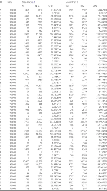
Table 3

(

Continued

)

NI NFG CPU NI NFG CPU

9 150,000 12 28 0.549281 3396 6792 140.188300

10 150,000 182 725 13.544060 178 709 13.124880

11 150,000 33 122 4.384094 46 137 4.963875

12 150,000 185 553 12.357280 1304 3837 85.495120

13 150,000 5 15 0.375813 78 233 5.665125

14 150,000 5317 21,266 1558.335000 1518 6035 435.598100

15 150,000 652 2597 43.007870 1510 5062 83.542500

16 150,000 4 8 0.327438 4 8 0.331625

17 150,000 4185 16,736 310.876300 4038 16,148 302.085700

18 150,000 577 2282 234.017300 651 2501 250.321700

19 150,000 543 2108 115.348700 606 2297 126.085400

20 150,000 1856 7388 108.733000 1201 4573 69.361500

21 150,000 37 114 3.196656 462 1385 41.271310

22 150,000 54 214 4.151344 54 214 4.162875

23 150,000 7833 15,670 463.476000 7796 15,596 470.208800

24 150,000 70 347 6.909438 697 3370 67.468870

25 150,000 911 4185 149.822700 1271 5619 200.791100

26 150,000 1088 5415 89.901440 24 114 1.983250

27 150,000 2215 11,021 35.738090 3730 18,481 62.137870

28 150,000 741 3672 64.568810 741 3672 65.072250

29 150,000 889 4377 121.323800 889 4377 121.201100

30 150,000 981 4890 125.251900 3772 18,694 85,912.53

31 150,000 24 94 0.809406 24 94 0.824999

32 150,000 26 77 1.310812 26 77 1.307996

33 150,000 14 67 3.713187 14 67 3.747922

34 150,000 703 3511 100.417200 1388 6145 186.073000

35 150,000 10,000 39,998 1754.543000 4503 17,809 787.514800

36 150,000 38 187 2.184250 38 187 2.263187

37 150,000 707 2369 118.873700 690 2315 118.594500

38 150,000 2 7 0.325656 2 7 0.332813

39 150,000 2880 14,397 587.451400 2879 14,392 606.360800

40 150,000 10,000 30,267 1747.903000 672 2196 113.973500

41 150,000 184 735 3.663625 694 2722 13.838310

42 150,000 1358 6771 22.041560 3702 18,337 202.568000

43 150,000 1210 6037 111.168500 4543 22,507 1077.162000

44 150,000 530 2101 102.349000 535 2115 109.978700

45 150,000 274 819 13.210880 1690 4988 98.434780

46 150,000 7 32 0.966938 7 32 1.057281

47 150,000 973 2918 34.427190 973 2918 38.767780

48 150,000 65 215 1.448500 646 1909 15.874250

49 150,000 2 7 0.331188 2 7 0.354250

50 150,000 1308 6537 263.783100 1311 6552 293.491800

51 150,000 7765 38,822 1684.177000 7766 38,827 1981.202000

52 150,000 10,000 30,268 1756.903000 644 2118 119.279600

53 150,000 2 7 0.324875 2 7 0.425313

54 150,000 7434 37,167 1561.060000 7434 37,167 1800.328000

55 150,000 2059 10,292 446.907300 2062 10,307 487.069700

56 150,000 1088 4350 20.671000 1088 4350 25.482500

57 150,000 2 6 0.030125 2 6 0.043125

58 150,000 28 83 2.166875 34 100 2.942250

59 150,000 540 1619 49.252810 541 1622 54.262940

60 150,000 1086 4341 253.299800 1114 4453 281.304400

61 150,000 2 7 0.314938 2 7 0.324813

62 150,000 65 215 1.469437 646 1909 15.412690

63 150,000 1 215 145.548700 1 1909 159.423600

64 150,000 10,000 49,809 196.063200 7233 35,833 189.318800

65 150,000 8676 43,204 140.774700 4592 22,753 93.901630

1 210,000 573 2836 122.895800 575 2844 123.117700

2 210,000 53 262 17.625310 56 277 19.078840

(21)

[image:21.595.121.478.114.723.2]

Table 3

(

Continued

)

NI NFG CPU NI NFG CPU

4 210,000 2053 8524 329.735100 2007 8265 363.818300

5 210,000 839 3263 42.105750 6047 23,976 318.768000

6 210,000 1385 6911 176.616000 3778 18,725 481.052400

7 210,000 195 972 32.574000 196 977 32.512590

8 210,000 195 584 11.812690 195 584 11.700880

9 210,000 10 25 0.636500 3828 7656 216.963400

10 210,000 151 601 15.601060 149 593 16.178340

11 210,000 35 133 7.425500 46 137 6.971656

12 210,000 159 475 14.729620 1457 4286 133.270000

13 210,000 7 21 0.690063 78 233 7.877844

14 210,000 5403 21,610 2218.623000 1531 6085 613.377000

15 210,000 1027 4086 95.329560 1527 5113 117.547900

16 210,000 4 8 0.469438 4 8 0.469063

17 210,000 4244 16,972 440.685700 4103 16,408 427.691300

18 210,000 578 2286 327.911200 651 2501 349.330900

19 210,000 543 2108 161.378500 606 2297 11,790.320000

20 210,000 2097 8332 171.760500 1201 4573 97.047560

21 210,000 41 129 5.103688 470 1409 58.391690

22 210,000 54 214 5.743125 54 214 5.820063

23 210,000 7833 15,670 654.266300 7796 15,596 652.518700

24 210,000 400 1997 55.551690 1261 6156 171.682500

25 210,000 1088 5415 125.671300 24 114 2.806562

26 210,000 2035 10,133 46.097440 3732 18,491 107.095900

27 210,000 686 3427 84.321690 686 3427 85.084120

28 210,000 872 4292 163.879400 872 4292 163.689200

29 210,000 1207 6011 219.317600 4992 24,796 874.306100

30 210,000 24 94 1.136250 24 94 1.203375

31 210,000 26 77 1.813437 26 77 1.918250

32 210,000 10 47 3.683844 10 47 3.776062

33 210,000 638 3187 127.252500 641 3202 127.119400

34 210,000 28 137 2.273625 28 137 2.449063

35 210,000 715 2393 169.418200 698 2339 164.307800

36 210,000 2 7 0.448313 2 7 0.455063

37 210,000 2880 14,397 825.603000 2879 14,392 829.216300

38 210,000 283 1131 7.781998 695 2725 20.372810

39 210,000 1240 6188 28.252000 3597 17,819 209.757800

40 210,000 1128 5627 145.184000 4559 22,590 1239.831000

41 210,000 371 1109 25.005980 1735 5125 127.223700

42 210,000 20 97 4.087996 19 92 4.170031

43 210,000 990 2969 49.404980 990 2969 49.341160

44 210,000 65 215 2.028015 646 1909 19.142310

45 210,000 2 7 0.452000 2 7 0.453688

46 210,000 1308 6537 368.925000 1311 6552 458.029900

47 210,000 7765 38,822 2364.621000 7766 38,827 3018.524000

48 210,000 10,000 30,268 2460.779000 676 2206 166.936300

49 210,000 2 7 0.467848 2 7 0.466844

50 210,000 7434 37,167 2191.087000 7434 37,167 3023.795000

51 210,000 2059 10,292 608.572100 2062 10,307 653.233600

52 210,000 1088 4350 28.642380 1088 4350 38.929310

53 210,000 2 6 0.030805 2 6 0.047719

54 210,000 34 102 3.696555 34 100 4.255938

55 210,000 548 1643 69.857270 549 1646 78.052220

56 210,000 1106 4421 360.469800 1130 4517 1023.525000

57 210,000 2 7 0.453117 2 7 0.492094

58 210,000 65 215 2.011992 646 1909 21.231910

59 210,000 1 215 285.122300 1 1909 318.237500

60 210,000 10,000 49,791 317.897200 7278 36,056 876.884300

(22)

Appendix 2

Table 4

Test problems

No. Problem

1 Generalization of MAXQ (convex) 2 Chained LQ (convex)

3 Number of active faces (nonconvex)

4 Nonsmooth generalization of Brown function (nonconvex) 5 Chained Miﬄin 2 (nonconvex)

[image:22.595.117.486.266.715.2]

6 Chained crescent (nonconvex) 7 Chained crescent 2 (nonconvex)

Table 5

Numerical results

NO Dim Algorithm3.1 Algorithm 2 Algorithm 3

NI NFG CPU NI NFG CPU NI NFG CPU

1 150,000 268 5592 27.595310 268 5592 27.707090 3 33 0.185438

2 150,000 67 173 1.497563 67 173 1.576625 137 312 2.091156

3 150,000 104 1808 24.912940 114 1836 25.536130 3 33 0.436469

4 150,000 75 185 20.279250 82 204 21.684970 137 313 35.800970

5 150,000 67 173 1.838000 67 173 1.873375 151 337 2.839188

6 150,000 55 205 1.859063 55 205 1.917375 137 312 2.385719

7 150,000 4 12 0.108688 4 12 0.108406 137 312 2.370000

1 180,000 271 5655 33.589060 271 5655 33.772090 3 33 0.218094

2 180,000 81 201 2.009625 81 201 2.059219 137 312 2.465594

3 180,000 109 1859 30.826380 116 1878 31.326120 3 33 0.483875

4 180,000 88 210 27.703250 93 225 28.768280 137 313 42.884500

5 180,000 81 201 2.465125 81 201 2.494750 151 337 3.402688

6 180,000 69 233 2.461375 69 233 2.510656 137 312 2.760719

7 180,000 5 15 0.172438 5 15 0.169938 137 312 2.776000

1 192,000 272 5676 36.939880 272 5676 37.251780 3 33 0.218531

2 192,000 72 176 1.889156 78 194 2.215563 137 312 2.744531

3 192,000 106 1850 34.069270 116 1878 35.289880 3 33 0.577375

4 192,000 90 216 30.327910 93 225 31.282190 137 313 45.879250

5 192,000 81 201 2.651781 81 201 2.855937 151 338 3.744344

6 192,000 69 233 2.651438 69 233 2.855469 137 312 3.040250

7 192,000 5 15 0.201094 5 15 0.187375 137 312 3.027188

1 210,000 273 5697 39.558750 273 5697 40.656190 3 33 0.249844

2 210,000 81 201 2.367750 81 201 2.449625 137 312 2.885844

3 210,000 109 1877 36.393310 117 1899 37.347190 3 33 0.578000

4 210,000 89 213 32.668690 96 232 34.631900 137 313 50.043880

5 210,000 81 201 2.836188 81 201 2.947094 151 338 3.995281

6 210,000 69 233 2.871250 69 233 2.946250 137 312 3.275187

7 210,000 5 15 0.198250 5 15 0.219938 137 312 3.246750

1 222,000 274 5718 41.885560 274 5718 42.759780 3 33 0.278094

2 222,000 70 170 2.013531 80 200 2.541594 137 312 3.026187

3 222,000 109 1877 38.548250 117 1899 39.467090 3 33 0.637906

4 222,000 96 232 37.098370 96 232 36.658720 137 313 53.057190

5 222,000 81 201 3.026719 81 201 3.106844 151 337 4.210594

6 222,000 69 233 3.041375 69 233 3.121375 137 312 3.478031

7 222,000 5 15 0.216406 5 15 0.218281 137 312 3.449469

1 231,000 275 5739 43.525590 275 5739 44.507000 3 33 0.265125

2 231,000 81 201 2.573875 79 197 2.604687 137 312 3.183219

3 231,000 118 1920 41.074940 118 1920 41.665530 3 33 0.625156

4 231,000 85 201 34.211090 96 232 38.190850 137 313 55.084160

5 231,000 81 201 3.151156 81 201 3.228437 151 337 4.366219

6 231,000 70 236 3.196813 70 236 3.324875 137 312 3.587406

(23)

[image:23.595.117.479.94.338.2]

Table 5

(

Continued

)

NO Dim Algorithm3.1 Algorithm 2 Algorithm 3

NI NFG CPU NI NFG CPU NI NFG CPU

1 240,000 275 5739 45.549500 275 5739 47.158840 3 33 0.279813

2 240,000 81 201 2.702625 81 201 2.777250 137 312 3.307688

3 240,000 107 1889 41.918190 118 1920 43.150280 3 33 0.655719

4 240,000 96 232 40.166310 96 232 39.578840 137 313 57.328840

5 240,000 81 201 3.278250 81 201 3.354719 151 337 4.555719

6 240,000 70 236 3.319375 70 236 3.431250 137 312 3.745031

7 240,000 4 12 0.171063 4 12 0.188563 137 312 3.727937

1 252,000 276 5760 47.984220 276 5760 51.422370 3 33 0.295813

2 252,000 72 176 2.386094 81 201 2.901656 137 312 3.430656

3 252,000 118 1920 44.880910 118 1920 45.349560 3 33 0.703563

4 252,000 96 232 42.087090 96 232 41.544910 137 313 60.076440

5 252,000 81 201 3.433156 81 201 3.526937 151 338 4.771313

6 252,000 70 236 3.478938 70 236 3.603594 137 312 3.901781

7 252,000 4 12 0.185469 4 12 0.185125 137 312 3.899437

1 270,000 277 5781 51.697340 277 5781 52.729160 3 33 0.327406

2 270,000 75 185 2.761375 80 200 3.089156 137 312 3.681875

3 270,000 110 1916 47.813940 119 1941 49.108690 3 33 0.733344

4 270,000 96 232 45.132440 96 232 44.506310 137 313 64.317340

5 270,000 81 201 3.681625 81 201 3.789500 151 337 5.117938

6 270,000 70 236 3.760937 70 236 3.869437 137 312 4.212750

7 270,000 4 12 0.202219 4 12 0.200344 137 312 4.197813

Acknowledgements

The authors would like to thank for the support funds.

Funding

This work was supported by the National Natural Science Foundation of China (Grant No. 11661009), the Guangxi Natural Science Fund for Distinguished Young Scholars (No. 2015GXNSFGA139001), and the Guangxi Natural Science Key Fund (No. 2017GXNSFDA198046).

Competing interests

The authors declare to have no competing interests.

Authors’ contributions

GY mainly analyzed the theory results and organized this paper, TL did the numerical experiments of smooth problems and WH focused on the nonsmooth problems and image problems. All authors read and approved the ﬁnal manuscript.

Publisher’s Note

Springer Nature remains neutral with regard to jurisdictional claims in published maps and institutional aﬃliations.

Received: 30 January 2019 Accepted: 27 August 2019

References

1. Al-Baali, A., Albaali, M.: Descent property and global convergence of the Fletcher–Reeves method with inexact line search. IMA J. Numer. Anal.5(1), 121–124 (1985)

2. Al-Baali, M., Narushima, Y., Yabe, H.: A family of three-term conjugate gradient methods with suﬃcient descent property for unconstrained optimization. Comput. Optim. Appl.60(1), 89–110 (2015)

3. Andrei, N.: An unconstrained optimization test functions collection. Environ. Sci. Technol.10(1), 6552–6558 (2008) 4. Andrei, N.: On three-term conjugate gradient algorithms for unconstrained optimization. Appl. Math. Comput.

241(11), 19–29 (2008)

<