Simulations of the formation, evolution and clustering of galaxies and quasars

arXiv:astro-ph/0504097v2 6 Apr 2005

Simulating the joint evolution of quasars, galaxies

and their large-scale distribution

Volker Springel1, Simon D. M. White1, Adrian Jenkins2, Carlos S. Frenk2, Naoki Yoshida3, Liang Gao1, Julio Navarro4, Robert Thacker5, Darren Croton1, John Helly2, John A. Peacock6, Shaun Cole2, Peter Thomas7, Hugh Couchman5, August Evrard8, J ¨org Colberg9 & Frazer Pearce10

1_{Max-Planck-Institute for Astrophysics, Karl-Schwarzschild-Str. 1, 85740 Garching, Germany}

2_{Inst. for Computational Cosmology, Dep. of Physics, Univ. of Durham, South Road, Durham DH1 3LE, UK} 3_{Department of Physics, Nagoya University, Chikusa-ku, Nagoya 464-8602, Japan}

4_{Dep. of Physics & Astron., University of Victoria, Victoria, BC, V8P 5C2, Canada}

5_{Dep. of Physics & Astron., McMaster Univ., 1280 Main St. West, Hamilton, Ontario, L8S 4M1, Canada} 6_{Institute of Astronomy, University of Edinburgh, Blackford Hill, Edinburgh EH9 3HJ, UK}

7_{Dep. of Physics & Astron., University of Sussex, Falmer, Brighton BN1 9QH, UK} 8_{Dep. of Physics & Astron., Univ. of Michigan, Ann Arbor, MI 48109-1120, USA}

9_{Dep. of Physics & Astron., Univ. of Pittsburgh, 3941 O’Hara Street, Pittsburgh PA 15260, USA} 10_{Physics and Astronomy Department, Univ. of Nottingham, Nottingham NG7 2RD, UK}

The cold dark matter model has become the leading theoretical paradigm for the

for-mation of structure in the Universe. Together with the theory of cosmic inflation, this

model makes a clear prediction for the initial conditions for structure formation and

predicts that structures grow hierarchically through gravitational instability. Testing

this model requires that the precise measurements delivered by galaxy surveys can be

compared to robust and equally precise theoretical calculations. Here we present a novel

framework for the quantitative physical interpretation of such surveys. This combines

the largest simulation of the growth of dark matter structure ever carried out with new

techniques for following the formation and evolution of the visible components. We show

that baryon-induced features in the initial conditions of the Universe are reflected in

dis-torted form in the low-redshift galaxy distribution, an effect that can be used to constrain

Recent large surveys such as the 2 degree Field Galaxy Redshift Survey (2dFGRS) and

the Sloan Digital Sky Survey (SDSS) have characterised much more accurately than ever

be-fore not only the spatial clustering, but also the physical properties of low-redshift galaxies.

Major ongoing campaigns exploit the new generation of 8m-class telescopes and the Hubble

Space Telescope to acquire data of comparable quality at high redshift. Other surveys target

the weak image shear caused by gravitational lensing to extract precise measurements of the

distribution of dark matter around galaxies and galaxy clusters. The principal goals of all these

surveys are to shed light on how galaxies form, to test the current paradigm for the growth of

cosmic structure, and to search for signatures which may clarify the nature of dark matter and

dark energy. These goals can be achieved only if the accurate measurements delivered by the

surveys can be compared to robust and equally precise theoretical predictions. Two problems

have so far precluded such predictions: (i) accurate estimates of clustering require simulations

of extreme dynamic range, encompassing volumes large enough to contain representative

pop-ulations of rare objects (like rich galaxy clusters or quasars), yet resolving the formation of

individual low luminosity galaxies; (ii) critical aspects of galaxy formation physics are

uncer-tain and beyond the reach of direct simulation (for example, the structure of the interstellar

medium, its consequences for star formation and for the generation of galactic winds, the

ejection and mixing of heavy elements, AGN feeding and feedback effects . . . ) – these must

be treated by phenomenological models whose form and parameters are adjusted by trial and

error as part of the overall data-modelling process. We have developed a framework which

combines very large computer simulations of structure formation with post-hoc modelling of

galaxy formation physics to offer a practical solution to these two entwined problems.

During the past two decades, the cold dark matter (CDM) model, augmented with a dark

the standard theoretical paradigm for galaxy formation. It assumes that structure grew from

weak density fluctuations present in the otherwise homogeneous and rapidly expanding early

universe. These fluctuations are amplified by gravity, eventually turning into the rich

struc-ture that we see around us today. Confidence in the validity of this model has been boosted

by recent observations. Measurements of the cosmic microwave background (CMB) by the

WMAP satellite1were combined with the 2dFGRS to confirm the central tenets of the model

and to allow an accurate determination of the geometry and matter content of the Universe

about 380 000 years after the Big Bang2. The data suggest that the early density fluctuations

were a Gaussian random field, as predicted by inflationary theory, and that the current energy

density is dominated by some form of dark energy. This analysis is supported by the apparent

acceleration of the current cosmic expansion inferred from studies of distant supernovae3, 4_{, as}

well as by the low matter density derived from the baryon fraction of clusters5_.

While the initial, linear growth of density perturbations can be calculated analytically, the

collapse of fluctuations and the subsequent hierarchical build-up of structure is a highly

non-linear process which is only accessible through direct numerical simulation6. The dominant

mass component, the cold dark matter, is assumed to be made of elementary particles that

cur-rently interact only gravitationally, so the collisionless dark matter fluid can be represented by

a set of discrete point particles. This representation as an N-body system is a coarse

approx-imation whose fidelity improves as the number of particles in the simulation increases. The

high-resolution simulation described here – dubbed the Millennium Simulation because of its

size – was carried out by the Virgo Consortium, a collaboration of British, German, Canadian,

and US astrophysicists. It follows N=21603≃1.0078×1010particles from redshift z=127

to the present in a cubic region 500 h−1Mpc on a side, where 1+z is the expansion factor of

With ten times as many particles as the previous largest computations of this kind7–9(see

Sup-plementary Information), it offers substantially improved spatial and time resolution within a

large cosmological volume. Combining this simulation with new techniques for following the

formation and evolution of galaxies, we predict the positions, velocities and intrinsic

proper-ties of all galaxies brighter than the Small Magellanic Cloud throughout volumes comparable

to the largest current surveys. Crucially, this also allows us to establish evolutionary links

between objects observed at different epochs. For example, we demonstrate that galaxies with

supermassive central black holes can plausibly form early enough in the standard cold dark

matter cosmology to host the first known quasars, and that these end up at the centres of rich

galaxy clusters today.

Dark matter halos and galaxies

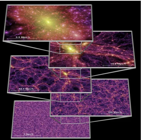
The mass distribution in a ΛCDM universe has a complex topology, often described as a

“cosmic web”10. This is visible in full splendour in Fig. 1 (see also the corresponding

Supple-mentary Video). The zoomed out panel at the bottom of the figure reveals a tight network of

cold dark matter clusters and filaments of characteristic size∼100 h−1Mpc. On larger scales,

there is little discernible structure and the distribution appears homogeneous and isotropic.

Subsequent images zoom in by factors of four onto the region surrounding one of the many

rich galaxy clusters. The final image reveals several hundred dark matter substructures,

re-solved as independent, gravitationally bound objects orbiting within the cluster halo. These

substructures are the remnants of dark matter halos that fell into the cluster at earlier times.

The space density of dark matter halos at various epochs in the simulation is shown in

Figure 1: The dark matter density field on various scales. Each individual image shows the projected

dark matter density field in a slab of thickness 15 h−1Mpc (sliced from the periodic simulation volume

1010 1011 1012 1013 1014 1015 1016 M [ h-1 MO • ]

10-5 10-4 10-3 10-2 10-1

M

2 /ρ

d

n

/d

M

z = 10.07

z = 5.72

z = 3.06

z = 1.50

z = 0.00

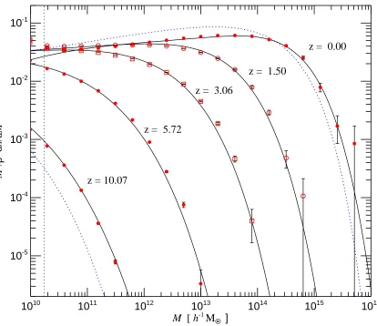
Figure 2: Differential halo number density as a function of mass and epoch. The function n(M,z)gives the comoving number density of halos less massive than M. We plot it as the halo multiplicity function

M2ρ−1dn/dM, where ρ is the mean density of the universe. Groups of particles were found using

a friends-of-friends algorithm6 with linking length equal to 0.2 of the mean particle separation. The

fraction of mass bound to halos of more than 20 particles (vertical dotted line) grows from 6.42×10−4

at z=10.07 to 0.496 at z=0. Solid lines are predictions from an analytic fitting function proposed in

most precise determination to date of the mass function of cold dark matter halos11, 12. In the

range that is well sampled in our simulation (z≤12, M≥1.7×1010h−1M⊙), our results are

remarkably well described by the analytic formula proposed by Jenkins et al.11 _{from fits to}

previous simulations. Theoretical models based on an ellipsoidal excursion set formulation13

give a less accurate, but still reasonable match. However, the commonly used Press-Schechter

formula14 underpredicts the high-mass end of the mass function by up to an order of

magni-tude. Previous studies of the abundance of rare objects, such as luminous quasars or clusters,

based on this formula may contain large errors15. We return below to the important question

of the abundance of quasars at early times.

To track the formation of galaxies and quasars in the simulation, we implement a

semi-analytic model to follow gas, star and supermassive black hole processes within the merger

history trees of dark matter halos and their substructures (see Supplementary Information).

The trees contain a total of about 800 million nodes, each corresponding to a dark matter

subhalo and its associated galaxies. This methodology allows us to test, during

postprocess-ing, many different phenomenological treatments of gas coolpostprocess-ing, star formation, AGN growth,

feedback, chemical enrichment, etc. Here, we use an update of models described in16, 17_which

are similar in spirit to previous semi-analytic models18–23_{; the modelling assumptions and}

pa-rameters are adjusted by trial and error in order to fit the observed properties of low redshift

galaxies, primarily their joint luminosity-colour distribution and their distributions of

mor-phology, gas content and central black hole mass. Our use of a high-resolution simulation,

particularly our ability to track the evolution of dark matter substructures, removes much of

the uncertainty of the more traditional semi-analytic approaches based on Monte-Carlo

real-izations of merger trees. Our technique provides accurate positions and peculiar velocities

objects and thus to investigate the relationship between populations seen at different epochs.

It is the ability to establish such evolutionary connections that makes this kind of modelling

so powerful for interpreting observational data.

The fate of the first quasars

Quasars are among the most luminous objects in the Universe and can be detected at huge

cosmological distances. Their luminosity is thought to be powered by accretion onto a central,

supermassive black hole. Bright quasars have now been discovered as far back as redshift

z=6.43 (ref. 24), and are believed to harbour central black holes of mass a billion times

that of the sun. At redshift z∼6, their comoving space density is estimated to be∼(2.2±

0.73)×10−9h3Mpc−3(ref.25_{). Whether such extreme rare objects can form at all in a}Λ_CDM

cosmology is an open question.

A volume the size of the Millennium Simulation should contain, on average, just under

one quasar at the above space density. Just what sort of object should be associated with these

“first quasars” is, however, a matter of debate. In the local universe, it appears that every bright

galaxy hosts a supermassive black hole and there is a remarkably good correlation between

the mass of the central black hole and the stellar mass or velocity dispersion of the bulge of

the host galaxy26_{. It would therefore seem natural to assume that at any epoch, the brightest}

quasars are always hosted by the largest galaxies. In our simulation, ‘large galaxies’ can be

identified in various ways, for example, according to their dark matter halo mass, stellar mass,

or instantaneous star formation rate. We have identified the 10 ‘largest’ objects defined in these

three ways at redshift z=6.2. It turns out that these criteria all select essentially the same

selected by star formation rate, but the 4 first-ranked galaxies are still amongst the 8 identified

according to the other 2 criteria.

In Figure 3, we illustrate the environment of a “first quasar” candidate in our simulation at

z=6.2. The object lies on one of the most prominent dark matter filaments and is surrounded

by a large number of other, much fainter galaxies. It has a stellar mass of 6.8×1010h−1M⊙,

the largest in the entire simulation at z=6.2, a dark matter virial mass of 3.9×1012h−1M⊙,

and a star formation rate of 235 M⊙yr−1. In the local universe central black hole masses are

typically∼1/1000 of the bulge stellar mass27, but in the model we test here these massive

early galaxies have black hole masses in the range 108−109M⊙, significantly larger than low

redshift galaxies of similar stellar mass. To attain the observed luminosities, they must convert

infalling mass to radiated energy with a somewhat higher efficiency than the∼0.1 c2expected

for accretion onto a non-spinning black hole.

Within our simulation we can readily address fundamental questions such as: “Where are

the descendants of the early quasars today?”, or “What were their progenitors?”. By tracking

the merging history trees of the host halos, we find that all our quasar candidates end up today

as central galaxies in rich clusters. For example, the object depicted in Fig. 3 lies, today, at the

centre of the ninth most massive cluster in the volume, of mass M=1.46×1015h−1M⊙. The

candidate with the largest virial mass at z=6.2 (which has stellar mass 4.7×1010h−1M⊙,

virial mass 4.85×1012h−1M⊙, and star formation rate 218 M⊙yr−1) ends up in the second

most massive cluster, of mass 3.39×1015h−1M⊙. Following the merging tree backwards in

time, we can trace our quasar candidate back to redshift z=16.7, when its host halo had a

mass of only 1.8×1010h−1M⊙. At this epoch, it is one of just 18 objects that we identify as

collapsed systems with≥20 particles. These results confirm the view that rich galaxy clusters

Figure 3: Environment of a ‘first quasar candidate’ at high and low redshifts. The two panels on the

left show the projected dark matter distribution in a cube of comoving sidelength 10 h−1_Mpc,

colour-coded according to density and local dark matter velocity dispersion. The panels on the right show the galaxies of the semi-analytic model overlayed on a gray-scale image of the dark matter density. The volume of the sphere representing each galaxy is proportional to its stellar mass, and the chosen colours

encode the restframe stellar B−V colour index. While at z=6.2 (top) all galaxies appear blue due

to ongoing star formation, many of the galaxies that have fallen into the rich cluster at z=0 (bottom)

lie in the regions where the first structures developed at high redshift. Thus, the best place

to search for the oldest stars in the Universe or for the descendants of the first supermassive

black holes is at the centres of present-day rich galaxy clusters.

The clustering evolution of dark matter and galaxies

The combination of a large-volume, high-resolution N-body simulation with realistic

mod-elling of galaxies enables us to make precise theoretical predictions for the clustering of

galax-ies as a function of redshift and intrinsic galaxy propertgalax-ies. These can be compared directly

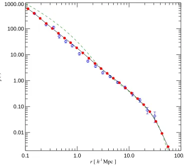
with existing and planned surveys. The 2-point correlation function of our model galaxies

at redshift z= 0 is plotted in Fig. 4 and is compared with a recent measurement from the

2dFGRS28_{. The prediction is remarkably close to a power-law, confirming with much higher}

precision the results of earlier semi-analytic23, 29_{and hydrodynamic}30_{simulations. This}

preci-sion will allow interpretation of the small, but measurable deviations from a pure power-law

found in the most recent data31, 32. The simple power-law form contrasts with the more

com-plex behaviour exhibited by the dark matter correlation function but is really no more than a

coincidence. Correlation functions for galaxy samples with different selection criteria or at

different redshifts do not, in general, follow power-laws.

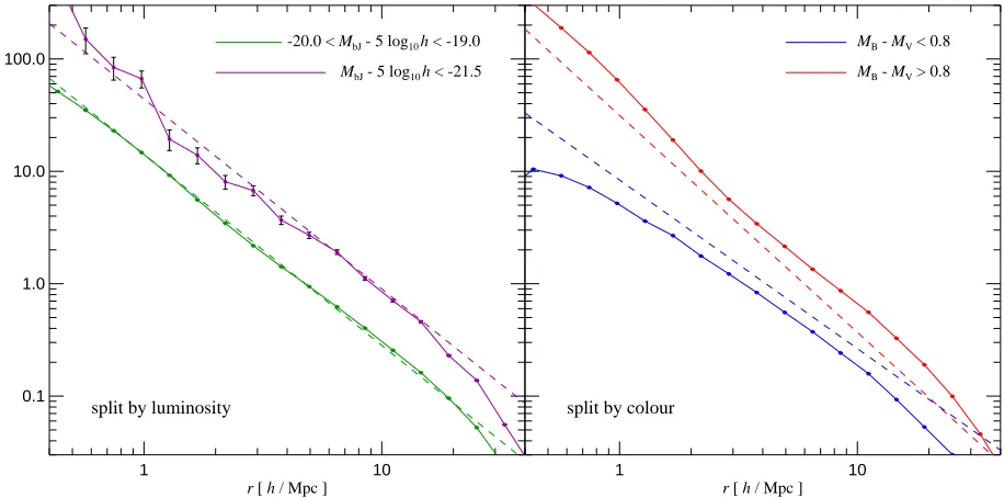
Although our semi-analytic model was not tuned to match observations of galaxy

clus-tering, in not only produces the excellent overall agreement shown in Fig. 4, but also

repro-duces the observed dependence of clustering on magnitude and colour in the 2dFGRS and

SDSS33–35, as shown in Figure 5. The agreement is particularly good for the dependence of

clustering on luminosity. The colour dependence of the slope is matched precisely, but the

amplitude difference is greater in our model than is observed35. Note that our predictions for

0.1 1.0 10.0 100.0 r [ h-1 Mpc ]

0.01 0.10 1.00 10.00 100.00 1000.00

ξ

(

r)

Figure 4: Galaxy 2-point correlation function at the present epoch. Red symbols (with vanishingly

small Poisson error-bars) show measurements for model galaxies brighter than MK=−23. Data for the

large spectroscopic redshift survey 2dFGRS28are shown as blue diamonds. The SDSS34and APM31

surveys give similar results. Both, for the observational data and for the simulated galaxies, the

corre-lation function is very close to a power-law for r≤20 h−1_{Mpc. By contrast the correlation function for}

1 10 r [ h / Mpc ] 0.1

1.0 10.0 100.0

ξ

(

r)

split by luminosity

-20.0 < MbJ - 5 log10h < -19.0 MbJ - 5 log10h < -21.5

1 10

r [ h / Mpc ]

MB - MV < 0.8

MB - MV > 0.8

split by colour

0.1

1.0

10.0

100.0

ξ

(r)

0.1

1.0

10.0

100.0

ξ

(r)

Figure 5: Galaxy clustering as a function of luminosity and colour. In the panel on the left, we show

the 2-point correlation function of our galaxy catalogue at z=0 split by luminosity in the bJ-band

(symbols). Brighter galaxies are more strongly clustered, in quantitative agreement with observations33

(dashed lines). Splitting galaxies according to colour (right panel), we find that red galaxies are more

strongly clustered with a steeper correlation slope than blue galaxies. Observations35 (dashed lines)

can be easily tested against survey data in order to clarify the physical processes responsible

for the observed difference.

In contrast to the near power-law behaviour of galaxy correlations on small scales, the

large-scale clustering pattern may show interesting structure. Coherent oscillations in the

pri-mordial plasma give rise to the well-known acoustic peaks in the CMB2, 36, 37 _{and also leave}

an imprint in the linear power spectrum of the dark matter. Detection of these “baryon

wig-gles” would not only provide a beautiful consistency check for the cosmological paradigm,

but could also have important practical applications. The characteristic scale of the wiggles

provides a “standard ruler” which may be used to constrain the equation of state of the dark

energy38_{. A critical question when designing future surveys is whether these baryon wiggles}

are present and are detectable in the galaxy distribution, particularly at high redshift.

On large scales and at early times, the mode amplitudes of the dark matter power spectrum

grow linearly, roughly in proportion to the cosmological expansion factor. Nonlinear evolution

accelerates the growth on small scales when the dimensionless power∆2(k) =k3P(k)/(2

π

approaches unity; this regime can only be studied accurately using numerical simulations. In

the Millennium Simulation, we are able to determine the nonlinear power spectrum over a

larger range of scales than was possible in earlier work39_{, almost five orders of magnitude in}

wavenumber k.

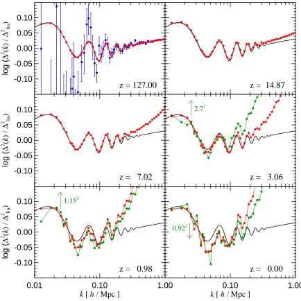
At the present day, the acoustic oscillations in the matter power spectrum are expected to

fall in the transition region between linear and nonlinear scales. In Fig. 6, we examine the

mat-ter power spectrum in our simulation in the region of the oscillations. Dividing by the smooth

power spectrum of aΛCDM model with no baryons40_{highlights the baryonic features in the}

number of large-scale modes. Since linear growth preserves the relative mode amplitudes,

we can approximately correct for this scatter by scaling the measured power in each bin by a

multiplicative factor based on the initial difference between the actual bin power and the mean

power expected in our ΛCDM model. This makes the effects of nonlinear evolution on the

baryon oscillations more clearly visible. As Fig. 6 shows, nonlinear evolution not only

accel-erates growth but also reduces the baryon oscillations: scales near peaks grow slightly more

slowly than scales near troughs. This is a consequence of the mode-mode coupling

character-istic of nonlinear growth. In spite of these effects, the first two “acoustic peaks” (at k∼0.07

and k∼0.13 h Mpc−1, respectively) in the dark matter distribution do survive in distorted form

until the present day (see the lower right panel of Fig. 6).

Are the baryon wiggles also present in the galaxy distribution? Fig. 6 shows that the

answer to this important question is ‘yes’. The z=0 panel shows the power spectrum for all

model galaxies brighter than MB=−17. On the largest scales, the galaxy power spectrum has

the same shape as that of the dark matter, but with slightly lower amplitude corresponding to

an “antibias” of 8%. Samples of brighter galaxies show less antibias while for the brightest

galaxies, the bias becomes slightly positive. The figure also shows measurements of the power

spectrum of luminous galaxies at redshifts z=0.98 and z=3.06. Galaxies at z=0.98 were

selected to have a magnitude MB<−19 in the restframe, whereas galaxies at z=3.06 were

selected to have stellar mass larger than 5.83×109h−1M⊙, corresponding to a space density of

8×10−3h3Mpc−3, similar to that of the Lyman-break galaxies observed at z∼341. Signatures

of the first two acoustic peaks are clearly visible at both redshifts, even though the density field

of the z=3 galaxies is much more strongly biased with respect to the dark matter (by a factor

b=2.7) than at low redshift. Selecting galaxies by their star formation rate rather than their

-0.10 -0.05 0.00 0.05 0.10 log ( ∆ 2 (k ) / ∆ 2 lin ) -0.10 -0.05 0.00 0.05 0.10 log ( ∆ 2(k) / ∆ 2lin)

0.01 0.10k [ h / Mpc ] 1.00

z = 127.00

-0.10 -0.05 0.00 0.05 0.10 log ( ∆ 2 ( k) / ∆ 2lin ) -0.10 -0.05 0.00 0.05 0.10 log ( ∆ 2(k) / ∆ 2lin)

0.01 0.10k [ h / Mpc ] 1.00

z = 14.87

-0.10 -0.05 0.00 0.05 0.10 log ( ∆ 2 (k ) / ∆ 2 lin ) -0.10 -0.05 0.00 0.05 0.10 log ( ∆ 2(k) / ∆ 2lin)

0.01 0.10k [ h / Mpc ] 1.00 0.01 0.10k [ h / Mpc ] 1.00

z = 7.02

-0.10 -0.05 0.00 0.05 0.10 log ( ∆ 2 ( k) / ∆ 2lin ) -0.10 -0.05 0.00 0.05 0.10 log ( ∆ 2(k) / ∆ 2lin)

0.01 0.10k [ h / Mpc ] 1.00 0.01 0.10k [ h / Mpc ] 1.00

2.72

z = 3.06

-0.10 -0.05 0.00 0.05 0.10 log ( ∆ 2 (k ) / ∆ 2 lin ) -0.10 -0.05 0.00 0.05 0.10 log ( ∆ 2(k) / ∆ 2lin)

0.01 0.10 1.00

k [ h / Mpc ]

0.01 0.10k [ h / Mpc ] 1.00

1.152

z = 0.98

-0.10 -0.05 0.00 0.05 0.10 log ( ∆ 2 ( k) / ∆ 2lin ) -0.10 -0.05 0.00 0.05 0.10 log ( ∆ 2(k) / ∆ 2lin) 0.10 1.00

k [ h / Mpc ]

0.1 1.0

k [ h / Mpc ]

0.922

z = 0.00

Figure 6: Power spectra of the dark matter and galaxy distributions in the baryon oscillation region.

All measurements have been divided by a linearly evolved, CDM-only power spectrum40. Red circles

show the dark matter, and green squares the galaxies. Blue symbols give the actual realization of the initial fluctuations in our simulation, which scatters around the mean input power (black lines) due to the finite number of modes. Since linear growth preserves relative mode amplitudes, we correct the power in each bin to the expected input power and apply these scaling factors at all other times. At

z=3.06, galaxies with stellar mass above 5.83×109h−1M⊙ and space-density of 8×10−3h3Mpc−3

were selected. Their large-scale density field is biased by a factor b=2.7 with respect to the dark

matter (the galaxy measurement has been divided by b2). At z=0, galaxies brighter than MB=−17

and a space density higher by a factor∼7.2 were selected. They exhibit a slight antibias, b=0.92.

results.

Our analysis demonstrates conclusively that baryon wiggles should indeed be present in

the galaxy distribution out to redshift z=3. This has been assumed but not justified in recent

proposals to use evolution of the large-scale galaxy distribution to constrain the nature of the

dark energy. To establish whether the baryon oscillations can be measured in practice with

the requisite accuracy will require detailed modelling of the selection criteria of an actual

sur-vey and a thorough understanding of the systematic effects that will inevitably be present in

real data. These issues can only be properly addressed by means of specially designed mock

catalogues constructed from realistic simulations. We plan to construct suitable mock

cata-logues from the Millennium Simulation and make them publicly available. Our provisional

conclusion, however, is that the next generation of galaxy surveys offers excellent prospects

for constraining the equation of state of the dark energy.

N-body simulations of CDM universes are now of such size and quality that realistic

modelling of galaxy formation in volumes matched to modern surveys has become possible.

Detailed studies of galaxy and AGN evolution exploiting the unique dataset of the Millennium

Simulation therefore enable stringent new tests of the theory of hierarchical galaxy formation.

Using the simulation we demonstrated that quasars can plausibly form sufficiently early in a

ΛCDM universe to be compatible with observation, that their progenitors were already

mas-sive by z∼16, and that their z=0 descendents lie at the centres of cD galaxies in rich galaxy

clusters. Interesting tests of our predictions will become possible if observations of the black

hole demographics can be extended to high redshift, allowing, for example, a measurement

of the evolution of the relationship between supermassive black hole masses and the velocity

We have also demonstrated that a power-law galaxy autocorrelation function can arise

naturally in aΛCDM universe, but that this suggestively simple behaviour is merely a

coin-cidence. Galaxy surveys will soon reach sufficient statistical power to measure precise

devia-tions from power-laws for galaxy subsamples, and we expect that comparisons of the kind we

have illustrated will lead to tight constraints on the physical processes included in the galaxy

formation modelling. Finally, we have demonstrated for the first time that the baryon-induced

oscillations recently detected in the CMB power spectrum should survive in distorted form not

only in the nonlinear dark matter power spectrum at low redshift, but also in the power spectra

of realistically selected galaxy samples at 0<z<3. Present galaxy surveys are marginally

able to detect the baryonic features at low redshifts42, 43_{. If future surveys improve on this and}

reach sufficient volume and galaxy density also at high redshift, then precision measurements

of galaxy clustering will shed light on one of the most puzzling components of the universe,

the elusive dark energy field.

Methods

The Millennium Simulation was carried out with a specially customised version of the

GAD-GET2(Ref. 44_{) code, using the “TreePM” method}45 _{for evaluating gravitational forces. This}

is a combination of a hierarchical multipole expansion, or “tree” algorithm46_{, and a classical,}

Fourier transform particle-mesh method47. The calculation was performed on 512 processors

of an IBM p690 parallel computer at the Computing Centre of the Max-Planck Society in

avail-The mean sustained floating point performance (as measured by hardware counters) was about

0.2 TFlops, so the total number of floating point operations carried out was of order 5×1017.

The cosmological parameters of our ΛCDM-simulation are: Ωm =Ωdm+Ωb =0.25,

Ωb =0.045, h=0.73, ΩΛ =0.75, n=1, and

σ

density in units of the critical density for closure,

ρ

π

denote the densities of baryons and dark energy at the present day. The Hubble constant is

parameterised as H0=100 h km s−1Mpc−1, while

σ

sphere of radius 8 h−1Mpc extrapolated to z=0. Our adopted parameter values are consistent

with a combined analysis of the 2dFGRS48 _{and first year WMAP data}2_.

The simulation volume is a periodic box of size 500 h−1Mpc and individual particles have

a mass of 8.6×108h−1M⊙. This volume is large enough to include interesting rare objects,

but still small enough that the halos of all luminous galaxies brighter than 0.1L⋆are resolved

with at least 100 particles. At the present day, the richest clusters of galaxies contain about

3 million particles. The gravitational force law is softened isotropically on a comoving scale

of 5 h−1kpc (Plummer-equivalent), which may be taken as the spatial resolution limit of the

calculation. Thus, our simulation achieves a dynamic range of 105 in 3D, and this resolution

is available everywhere in the simulation volume.

Initial conditions were laid down by perturbing a homogeneous, ‘glass-like’, particle

distribution49 with a realization of a Gaussian random field with the ΛCDM linear power

spectrum as given by the Boltzmann code CMBFAST50. The displacement field in Fourier

space was constructed using the Zel’dovich approximation, with the amplitude of each random

phase mode drawn from a Rayleigh distribution. The simulation started at redshift z=127

adap-tive timesteps, with up to 11 000 timesteps for individual particles. We stored the full particle

data at 64 output times, each of size 300 GB, giving a raw data volume of nearly 20 TB. This

allowed the construction of finely resolved hierarchical merging trees for tens of millions of

halos and for the subhalos that survive within them. A galaxy catalogue for the full simulation,

typically containing∼2×106galaxies at z=0 together with their full histories, can then be

built for any desired semi-analytic model in a few hours on a high-end workstation.

The semi-analytic model itself can be viewed as a simplified simulation of the galaxy

for-mation process, where the star forfor-mation and its regulation by feedback processes is

parame-terised in terms of simple analytic physical models. These models take the form of differential

equations for the time evolution of the galaxies that populate each hierarchical merging tree.

In brief, these equations describe radiative cooling of gas, star formation, growth of

supermas-sive black holes, feedback processes by supernovae and AGN, and effects due to a reionising

UV background. In addition, the morphological transformation of galaxies and the process of

metal enrichment are modelled as well. To make direct contact with observational data, we

apply modern population synthesis models to predict spectra and magnitudes for the stellar

light emitted by galaxies, also including simplified models for dust obscuration. In this way

we can match the passbands commonly used in observations.

The basic elements of galaxy formation modelling follow previous studies16, 18–23_{(see also}

Supplementary Information), but we also use novel approaches in a number of areas. Of

sub-stantial importance is our tracking of dark matter substructure. This we carry out consistently

and with unprecedented resolution throughout our large cosmological volume, allowing an

accurate determination of the orbits of galaxies within larger structures, as well as robust

of galactic disks and their rotation curves. Secondly, we employ a novel model for the

build-up of a population of sbuild-upermassive black holes in the universe. To this end we extend the

quasar model developed in previous work17 _{with a ‘radio mode’, which describes the}

feed-back activity of central AGN in groups and clusters of galaxies. While largely unimportant for

the cumulative growth of the total black hole mass density in the universe, our results show

that the radio mode becomes important at low redshift, where it has a strong impact on cluster

cooling flows. As a result, it reduces the brightness of central cluster galaxies, an effect that

shapes the bright end of the galaxy luminosity function, bringing our predictions into good

agreement with observation.

References

1. Bennett, C. L. et al. First-Year Wilkinson Microwave Anisotropy Probe (WMAP)

Obser-vations: Preliminary Maps and Basic Results. Astrophys. J. Suppl. 148, 1–27 (2003).

2. Spergel, D. N. et al. First-Year Wilkinson Microwave Anisotropy Probe (WMAP)

Obser-vations: Determination of Cosmological Parameters. Astrophys. J. Suppl. 148, 175–194

(2003).

3. Riess, A. G. et al. Observational Evidence from Supernovae for an Accelerating Universe

and a Cosmological Constant. Astron. J. 116, 1009–1038 (1998).

4. Perlmutter, S. et al. Measurements of Omega and Lambda from 42 High-Redshift

Super-novae. Astrophys. J. 517, 565–586 (1999).

5. White, S. D. M., Navarro, J. F., Evrard, A. E. & Frenk, C. S. The Baryon Content of

6. Davis, M., Efstathiou, G., Frenk, C. S. & White, S. D. M. The evolution of large-scale

structure in a universe dominated by cold dark matter. Astrophys. J. 292, 371–394 (1985).

7. Colberg, J. M. et al. Clustering of galaxy clusters in cold dark matter universes. Mon.

Not. R. Astron. Soc. 319, 209–214 (2000).

8. Evrard, A. E. et al. Galaxy Clusters in Hubble Volume Simulations: Cosmological

Con-straints from Sky Survey Populations. Astrophys. J. 573, 7–36 (2002).

9. Wambsganss, J., Bode, P. & Ostriker, J. P. Giant Arc Statistics in Concord with a

Concor-dance Lambda Cold Dark Matter Universe. Astrophys. J. Let. 606, L93–L96 (2004).

10. Bond, J. R., Kofman, L. & Pogosyan, D. How filaments of galaxies are woven into the

cosmic web. Nature 380, 603 (1996).

11. Jenkins, A. et al. The mass function of dark matter haloes. Mon. Not. R. Astron. Soc. 321,

372–384 (2001).

12. Reed, D. et al. Evolution of the mass function of dark matter haloes. Mon. Not. R. Astron.

Soc. 346, 565–572 (2003).

13. Sheth, R. K. & Tormen, G. An excursion set model of hierarchical clustering: ellipsoidal

collapse and the moving barrier. Mon. Not. R. Astron. Soc. 329, 61–75 (2002).

14. Press, W. H. & Schechter, P. Formation of Galaxies and Clusters of Galaxies by

Self-Similar Gravitational Condensation. Astrophys. J. 187, 425–438 (1974).

16. Springel, V., White, S. D. M., Tormen, G. & Kauffmann, G. Populating a cluster of

galaxies - I. Results at z=0. Mon. Not. R. Astron. Soc. 328, 726–750 (2001).

17. Kauffmann, G. & Haehnelt, M. A unified model for the evolution of galaxies and quasars.

Mon. Not. R. Astron. Soc. 311, 576–588 (2000).

18. White, S. D. M. & Frenk, C. S. Galaxy formation through hierarchical clustering.

Astro-phys. J. 379, 52–79 (1991).

19. Kauffmann, G., White, S. D. M. & Guiderdoni, B. The Formation and Evolution of

Galaxies Within Merging Dark Matter Haloes. Mon. Not. R. Astron. Soc. 264, 201–218

(1993).

20. Cole, S., Aragon-Salamanca, A., Frenk, C. S., Navarro, J. F. & Zepf, S. E. A Recipe for

Galaxy Formation. Mon. Not. R. Astron. Soc. 271, 781–806 (1994).

21. Baugh, C. M., Cole, S. & Frenk, C. S. Evolution of the Hubble sequence in hierarchical

models for galaxy formation. Mon. Not. R. Astron. Soc. 283, 1361–1378 (1996).

22. Somerville, R. S. & Primack, J. R. Semi-analytic modelling of galaxy formation: the

local Universe. Mon. Not. R. Astron. Soc. 310, 1087–1110 (1999).

23. Kauffmann, G., Colberg, J. M., Diaferio, A. & White, S. D. M. Clustering of galaxies

in a hierarchical universe - I. Methods and results at z=0. Mon. Not. R. Astron. Soc. 303,

188–206 (1999).

24. Fan, X. et al. A Survey of z>5.7 Quasars in the Sloan Digital Sky Survey. II. Discovery

of Three Additional Quasars at z>6. Astron. J. 125, 1649–1659 (2003).

25. Fan, X. et al. A Survey of z>5.7 Quasars in the Sloan Digital Sky Survey. III. Discovery

26. Tremaine, S. et al. The Slope of the Black Hole Mass versus Velocity Dispersion

Corre-lation. Astrophys. J. 574, 740–753 (2002).

27. Merritt, D. & Ferrarese, L. Black hole demographics from the MBH-

σ

R. Astron. Soc. 320, L30–L34 (2001).

28. Hawkins, E. et al. The 2dF Galaxy Redshift Survey: correlation functions, peculiar

ve-locities and the matter density of the Universe. Mon. Not. R. Astron. Soc. 346, 78–96

(2003).

29. Benson, A. J., Cole, S., Frenk, C. S., Baugh, C. M. & Lacey, C. G. The nature of galaxy

bias and clustering. Mon. Not. R. Astron. Soc. 311, 793–808 (2000).

30. Weinberg, D. H., Dav´e, R., Katz, N. & Hernquist, L. Galaxy Clustering and Galaxy Bias

in aΛCDM Universe. Astrophys. J. 601, 1–21 (2004).

31. Padilla, N. D. & Baugh, C. M. The power spectrum of galaxy clustering in the APM

Survey. Mon. Not. R. Astron. Soc. 343, 796–812 (2003).

32. Zehavi, I. et al. On Departures from a Power Law in the Galaxy Correlation Function.

Astrophys. J. 608, 16–24 (2004).

33. Norberg, P. et al. The 2dF Galaxy Redshift Survey: luminosity dependence of galaxy

clustering. Mon. Not. R. Astron. Soc. 328, 64–70 (2001).

34. Zehavi, I. et al. Galaxy Clustering in Early Sloan Digital Sky Survey Redshift Data.

Astrophys. J. 571, 172–190 (2002).

36. de Bernardis, P. et al. A flat Universe from high-resolution maps of the cosmic microwave

background radiation. Nature 404, 955–959 (2000).

37. Mauskopf, P. D. et al. Measurement of a Peak in the Cosmic Microwave Background

Power Spectrum from the North American Test Flight of Boomerang. Astrophys. J. Let.

536, L59–L62 (2000).

38. Blake, C. & Glazebrook, K. Probing Dark Energy Using Baryonic Oscillations in the

Galaxy Power Spectrum as a Cosmological Ruler. Astrophys. J. 594, 665–673 (2003).

39. Jenkins, A. et al. Evolution of Structure in Cold Dark Matter Universes. Astrophys. J.

499, 20–40 (1998).

40. Bardeen, J. M., Bond, J. R., Kaiser, N. & Szalay, A. S. The statistics of peaks of Gaussian

random fields. Astrophys. J. 304, 15–61 (1986).

41. Adelberger, K. L. et al. A Counts-in-Cells Analysis Of Lyman-break Galaxies At Redshift

Z ˜ 3. Astrophys. J. 505, 18–24 (1998).

42. Cole, S. et al. The 2dF Galaxy Redshift Survey: Power-spectrum analysis of the

fi-nal dataset and cosmological implications. Mon. Not. R. Astron. Soc. submitted, astro–

ph/0501174 (2005).

43. Eisenstein, D. J. et al. The 2dF Galaxy Redshift Survey: Power-spectrum analysis of the

final dataset and cosmological implications. Astrophys. J. submitted, astro–ph/0501171

(2005).

44. Springel, V., Yoshida, N. & White, S. D. M. GADGET: a code for collisionless and

45. Xu, G. A New Parallel N-Body Gravity Solver: TPM. Astrophys. J. Suppl. 98, 355–366

(1995).

46. Barnes, J. & Hut, P. A Hierarchical O(NlogN) Force-Calculation Algorithm. Nature 324,

446–449 (1986).

47. Hockney, R. W. & Eastwood, J. W. Computer Simulation Using Particles (New York:

McGraw-Hill, 1981, 1981).

48. Colless, M. et al. The 2dF Galaxy Redshift Survey: spectra and redshifts. Mon. Not. R.

Astron. Soc. 328, 1039–1063 (2001).

49. White, S. D. M. Formation and evolution of galaxies: Les houches lectures. In

Schae-fer, R., Silk, J., Spiro, M. & Zinn-Justin, J. (eds.) Cosmology and Large-Scale Structure

(Dordrecht: Elsevier, astro-ph/9410043, 1996).

50. Seljak, U. & Zaldarriaga, M. A Line-of-Sight Integration Approach to Cosmic Microwave

Background Anisotropies. Astrophys. J. 469, 437–444 (1996).

Supplementary Information accompanies the paper on www.nature.com/nature.

Acknowledgements We would like to thank the anonymous referees who helped to

im-prove the paper substantially. The computations reported here were performed at the

Rechen-zentrum der Max-Planck-Gesellschaft in Garching, Germany.

Competing interests The authors declare that they have no competing financial interests.

Correspondence and requests for materials should be addressed to V.S. (email:

Simulating the joint evolution of quasars, galaxies

and their large-scale distribution

Supplementary Information

V. Springel1, S. D. M. White1, A. Jenkins2, C. S. Frenk2, N. Yoshida3, L. Gao1, J. Navarro4_{, R. Thacker}5_{, D. Croton}1_{, J. Helly}2_{, J. A. Peacock}6_{, S. Cole}2_, P. Thomas7_{, H. Couchman}5_{, A. Evrard}8_{, J. Colberg}9_{& F. Pearce}10

This document provides supplementary infor-mation for the above article in Nature. We detail the physical model used to compute the galaxy population, and give a short summary of our simulation method. Where appropriate, we give further references to relevant literature for our methodology.

Characteristics of the simulation

Numerical simulations are a primary theoretical tool to study the nonlinear gravitational growth of struc-ture in the Universe, and to link the initial condi-tions of cold dark matter (CDM) cosmogonies to ob-servations of galaxies at the present day. Without

1_{Max-Planck-Institute for Astrophysics,}

Karl-Schwarzschild-Str. 1, 85740 Garching, Germany

2_{Institute for Computational Cosmology, Dep. of}

Physics, Univ. of Durham, South Road, Durham DH1 3LE, UK

3_{Department of Physics, Nagoya University,}

Chikusa-ku, Nagoya 464-8602, Japan

4_{Dep. of Physics & Astron., University of Victoria,}

Vic-toria, BC, V8P 5C2, Canada

5_{Dep. of Physics & Astron., McMaster Univ., 1280}

Main St. West, Hamilton, Ontario, L8S 4M1, Canada

6_{Institute of Astronomy, University of Edinburgh,}

Blackford Hill, Edinburgh EH9 3HJ, UK

7_{Dep. of Physics & Astron., University of Sussex,}

Falmer, Brighton BN1 9QH, UK

8_{Dep. of Physics & Astron., Univ. of Michigan, Ann}

Arbor, MI 48109-1120, USA

9_{Dep. of Physics & Astron., Univ. of Pittsburgh, 3941}

O’Hara Street, Pittsburgh PA 15260, USA

10_{Physics and Astronomy Department, Univ. of}

Notting-direct numerical simulation, the hierarchical build-up of structure with its three-dimensional dynamics would be largely inaccessible.

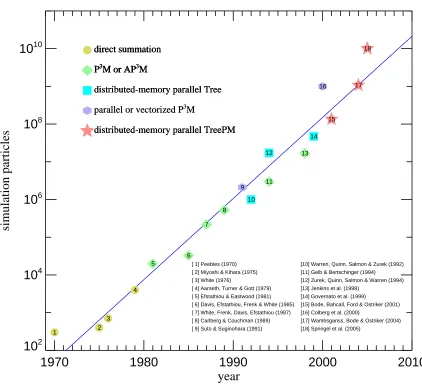
Since the dominant mass component, the dark matter, is assumed to consist of weakly interacting elementary particles that interact only gravitation-ally, such simulations use a set of discrete point par-ticles to represent the collisionless dark matter fluid. This representation as an N-body system is obvi-ously only a coarse approximation, and improving its fidelity requires the use of as many particles as possi-ble while remaining computationally tractapossi-ble. Cos-mological simulations have therefore always striven to increase the size (and hence resolution) of N-body computations, taking advantage of every ad-vance in numerical algorithms and computer hard-ware. As a result, the size of simulations has grown continually over the last four decades. Fig. 7 shows the progress since 1970. The number of particles has increased exponentially, doubling roughly ev-ery 16.5 months. Interestingly, this growth paral-lels the empirical ‘Moore’s Law’ used to describe the growth of computer performance in general. Our new simulation discussed in this paper uses an

un-precedentedly large number of 21603particles, more

than 1010. We were able to finish this computation

the remarkable progress since the 1970s for another three decades, we may expect cosmological

simula-tions with∼1020 particles some time around 2035.

This would be sufficient to represent all stars in a region as large as the Millennium volume with indi-vidual particles.

Initial conditions. We used the Boltzmann code

CMBFAST24to compute a linear theory power

spec-trum of aΛCDM model with cosmological

parame-ters consistent with recent constraints from WMAP

and large-scale structure data25, 26. We then

con-structed a random realization of the model in Fourier space, sampling modes in a sphere up to the Nyquist

frequency of our 21603 particle load. Mode

am-plitudes |δk|were determined by random sampling

from a Rayleigh distribution with second moment

equal to P(k) =

|δk|2

, while phases were cho-sen randomly. A high quality random number

gen-erator with period ∼10171 was used for this

pur-pose. We employed a massively parallel complex-to-real Fourier transform (which requires some care to satisfy all reality constraints) to directly obtain the resulting displacement field in each dimension. The initial displacement at a given particle coordi-nate of the unperturbed density field was obtained by tri-linear interpolation of the resulting displace-ment field, with the initial velocity obtained from the Zel’dovich approximation. The latter is very

accu-rate for our starting redshift of z=127. For the

ini-tial unperturbed density field of 21603 particles we

used a glass-like particle distribution. Such a glass is formed when a Poisson particle distribution in a periodic box is evolved with the sign of gravity re-versed until residual forces have dropped to

negligi-ble levels27. For reasons of efficiency, we replicated

a 2703glass file 8 times in each dimension to

gener-ate the initial particle load. The Fast Fourier Trans-forms (FFT) required to compute the displacement

fields were carried out on a 25603 mesh using 512

processors and a distributed-memory code. We de-convolved the input power spectrum for smoothing effects due to the interpolation off this grid.

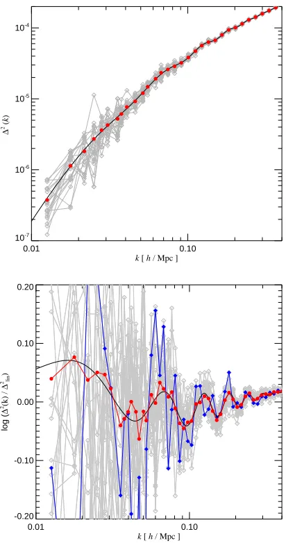
We note that the initial random number seed was picked in an unconstrained fashion. Due to the finite

0.01 0.10

k [ h / Mpc ]

10-7

10-6

10-5

10-4

∆

2 (

k)

0.01 0.10

k [ h / Mpc ]

-0.20 -0.10 0.00 0.10 0.20 log ( ∆

2(k) /

∆

2 lin

)

Figure 8: Different realizations of the initial power

spectrum. The top and bottom panels show mea-sured power-spectra for 20 realizations of initial con-ditions with different random number seeds, together

with the mean spectrum (red symbols). The

lat-ter lies close to the input linear power spectrum (black solid line). In the bottom panel, the mea-surements have been divided by a smooth CDM-only

power spectrum23 to highlight the acoustic

1970

1980

1990

2000

2010

year

10

10

10

10

10

simulation particles

P3M or AP3M

5

P3M or AP3M

6

P3M or AP3M

7

P3M or AP3M

8

parallel or vectorized P3_M

9

distributed-memory parallel Tree

10

P3M or AP3M

11

distributed-memory parallel Tree

12

P3M or AP3M

13

distributed-memory parallel Tree

14

distributed-memory parallel TreePM

15

parallel or vectorized P3_M

16

distributed-memory parallel TreePM

17

distributed-memory parallel TreePM

18

[ 1] Peebles (1970) [ 2] Miyoshi & Kihara (1975) [ 3] White (1976)

[ 4] Aarseth, Turner & Gott (1979) [ 5] Efstathiou & Eastwood (1981) [ 6] Davis, Efstathiou, Frenk & White (1985) [ 7] White, Frenk, Davis, Efstathiou (1987) [ 8] Carlberg & Couchman (1989) [ 9] Suto & Suginohara (1991)

[10] Warren, Quinn, Salmon & Zurek (1992) [11] Gelb & Bertschinger (1994) [12] Zurek, Quinn, Salmon & Warren (1994) [13] Jenkins et al. (1998)

[14] Governato et al. (1999)

[15] Bode, Bahcall, Ford & Ostriker (2001) [16] Colberg et al. (2000)

[17] Wambsganss, Bode & Ostriker (2004) [18] Springel et al. (2005)

Figure 7: Particle number in high resolution N-body simulations of cosmic structure formation as a function

of publication date1–17. Over the last three decades, the growth in simulation size has been exponential,

doubling approximately every∼16.5 months (blue line). Different symbols are used for different classes

of computational algorithms. The particle-mesh (PM) method combined with direct particle-particle (PP) summation on sub-grid scales has long provided the primary path towards higher resolution. However, due to their large dynamic range and flexibility, tree algorithms have recently become competitive with these

traditional P3M schemes, particularly if combined with PM methods to calculate the long-range forces. Plain

PM simulations18–22have not been included in this overview because of their much lower spatial resolution

is biased low due to the skew-negative distribution of the mode amplitudes. Hence, in a given realiza-tion there are typically more points lying below the input power spectrum than above it, an effect that quickly becomes negligible as the number of inde-pendent modes in each bin becomes large. We illus-trate this in the top panel of Figure 8, where 20 re-alizations for different random number seeds of the power spectrum on large scales are shown, together with the average power in each bin. Our particu-lar realization for the Millennium Simulation corre-sponds to a slightly unlucky choice of random num-ber seed in the sense that the fluctuations around the mean input power in the region of the second peak seem to resemble the pattern of the acoustic oscilla-tions (see the top left panel of Figure 6 in our Nature article). However, we stress that the fluctuations in these bins are random and uncorrelated, and that this impression is only a chance effect. In the bottom panel of Figure 8, we redraw the measured power spectra for the 20 random realizations, this time nor-malised to a smooth CDM power spectrum without acoustic oscillations in order to highlight the bary-onic ‘wiggles’. We have drawn one of the 20 realiza-tions in blue. It is one that resembles the pattern of fluctuations seen in the Millennium realization quite closely while others scatter quite differently, show-ing that such deviations are consistent with the ex-pected statistical distribution.

Dynamical evolution. The evolution of the

sim-ulation particles under gravity in an expanding back-ground is governed by the Hamiltonian

H=

∑

i

p2_i

2 mia(t)2

+1

2

∑

mimjϕ(xi−xj)

a(t) , (1)

where H =H(p1, . . . ,pN,x1, . . . ,xN,t). The xi are

comoving coordinate vectors, and the corresponding

canonical momenta are given by pi =a2mi˙xi. The

explicit time dependence of the Hamiltonian arises

from the evolution a(t) of the scale factor, which

is given by the Friedman-Lemaitre model that de-scribes the background cosmology. Due to our as-sumption of periodic boundary conditions for a cube

of size L3, the interaction potentialϕ(x)is the

solu-tion of

where the sum over n= (n1,n2,n3)extends over all

integer triplets. The density distribution function

δε(x)of a single particle is spread over a finite scale

ε, the gravitational softening length. The softening is

necessary to make it impossible for hard binaries to form and to allow the integration of close particle en-counters with low-order integrators. We use a spline

kernel to soften the point mass, given by δε(x) =

W(|x|/2.8ε), where W(r) =8(1−6r2+6r3)/π for

0≤r<1/2, W(r) =16(1−r)3_/π _{for 1/2≤r<}

1, and W(r) =0 otherwise. For this choice, the

Newtonian potential of a point mass at zero lag in

non-periodic space is −G m/ε, the same as for a

‘Plummer-sphere’ of size ε, and the force becomes

fully Newtonian for separations larger than 2.8ε. We

tookε=5 h−1kpc, about 46.3 times smaller than the

mean particle separation. Note that the mean density is subtracted in equation (2), so the solution of the Poisson equation corresponds to the peculiar

poten-tial, where the dynamics of the system is governed

by∇2φ(x) =4πG[ρ(x)−ρ].

The equations of motion corresponding to

equa-tion (1) are ∼1010 simple differential equations,

which are however coupled tightly by the mutual gravitational forces between the particles. An ac-curate evaluation of these forces (the ‘right hand side’ of the equations) is computationally very

ex-pensive, even when force errors up to ∼1% can

be tolerated, which is usually the case in

collision-less dynamics28. We have written a completely

new version of the cosmological simulation code

GADGET29 for this purpose. Our principal

com-putational technique for the gravitational force

cal-culation is a variant of the ‘TreePM’ method30–32,

which uses a hierarchical multipole expansion33 (a

‘tree’ algorithm) to compute short-range gravita-tional forces and combines this with a more

tra-ditional particle-mesh (PM) method34 to determine

long-range gravitational forces. This combination al-lows for a very large dynamic range and high com-putational speed even in situations where the clus-tering becomes strong. We use an explicit

force-split32 in Fourier-space, which produces a highly

opera-lation of the size and computational cost of the Mil-lennium Run.

For the tree-algorithm, we first decompose the simulation volume spatially into compact domains, each served by one processor. This domain decom-position is done by dividing a space filling Peano-Hilbert curve into segments. This fractal curve visits

each cell of a fiducial grid of 10243 cells overlayed

over the simulation exactly once. The decomposi-tion tries to achieve a work-load balance for each processor, and evolves over time as clustering pro-gresses. Using the Peano-Hilbert curve guarantees that domain boundaries are always parallel to natural tree-node boundaries, and thanks to its fractal nature provides for a small surface-to-volume ratio for all domains, such that communication with neighbour-ing processors durneighbour-ing the short-range tree force com-putation can be minimised. Our tree is fully threaded (i.e. its leaves are single particles), and implements an oct-tree structure with monopole moments only.

The cell-opening criterion was relative35_{; a multipole}

approximation was accepted if its conservatively

es-timated error was below 0.5% of the total force from

the last timestep. In addition, nodes were always opened when the particle under consideration lay in-side a 10% enlarged outer node boundary. This pro-cedure gives forces with typical errors well below

0.1%.

For the PM algorithm, we use a parallel Fast

Fourier Transform (FFT)∗ to solve Poisson’s

equa-tion. We used a FFT mesh with 25603 cells,

dis-tributed into 512 slabs of dimension 5×2560×2560

for the parallel transforms. After clouds-in-cells

(CIC) mass assignment to construct a density field, we invoke a real-to-complex transform to convert to Fourier space. We then multiplied by the Greens function of the Poisson equation, deconvolved for the effects of the CIC and the trilinear interpolation that is needed later, and applied the short-range fil-tering factor used in our TreePM formulation (the short range forces suppressed here are exactly those

supplied by the tree-algorithm). Upon

transform-ing back we obtained the gravitational potential. We then applied a four-point finite differencing formula to compute the gravitational force field for each of the three coordinate directions. Finally, the forces at each particle’s coordinate were obtained by trilinear

interpolation from these fields.

A particular challenge arises due to the differ-ent data layouts needed for the PM and tree algo-rithms. In order to keep the required communication and memory overhead low, we do not swap the par-ticle data between the domain and slab decomposi-tions. Instead, the particles stay in the domain de-composition needed by the tree, and each processor constructs patches of the density field for all the slabs on other processors which overlap its local domain. In this way, each processor communicates only with a small number of other processors to establish the binned density field on the slabs. Likewise, the slab-decomposed potential field is transfered back to pro-cessors so that a local region is formed covering the local domain, in addition to a few ghost cells around it, such that the finite differencing of the potential can be carried out for all interior points.

Timestepping was achieved with a symplectic leap-frog scheme based on a split of the potential energy into a short-range and long-range compo-nent. The short-range dynamics was then integrated

by subcycling the long-range step36. Hence, while

the short-range force had to be computed frequently, the long-range FFT force was needed only compar-atively infrequently. More than 11000 timesteps in total were carried out for the simulation, using

indi-vidual and adaptive timesteps† for the particles. A

timestep of a particle was restricted to be smaller

than∆t=p

2ηε/|a|, where a is a particle’s

acceler-ation andη=0.02 controls the integration accuracy.

We used a binary hierarchy of timesteps to generate a grouping of particles onto timebins.

The memory requirement of the code had to be aggressively optimised in order to make the simula-tion possible on the IBM p690 supercomputer avail-able to us. The total aggregated memory on the 512 processors was 1 TB, of which about 950 GB could be used freely by an application program. In our code Lean-GADGET-2 produced for the Millennium Simulation, we needed about 400 GB for particle storage and 300 GB for the fully threaded tree in the final clustered particle state, while the PM algorithm consumed in total about 450 GB in the final state

†_{Allowing adaptive changes of timesteps formally}

dy-0.01 0.10 1.00 10.00 100.00

k [ h / Mpc ]

10-4

10-3

10-2

10-1

100

101

102

103

104

∆

2 (

k)

z = 0.00

z = 0.98

z = 3.05

z = 7.02

z = 14.87

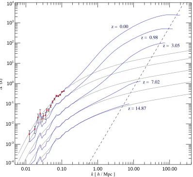
Figure 9: The power spectrum of the dark matter distribution in the Millennium Simulation at various

epochs (blue lines). The gray lines show the power spectrum predicted for linear growth, while the dashed line denotes the shot-noise limit expected if the simulation particles are a Poisson sampling from a smooth underlying density field. In practice, the sampling is significantly sub-Poisson at early times and in low density regions, but approaches the Poisson limit in nonlinear structures. Shot-noise subtraction allows us to probe the spectrum slightly beyond the Poisson limit. Fluctuations around the linear input spectrum on the largest scales are due to the small number of modes sampled at these wavelengths and the Rayleigh distribution of individual mode amplitudes assumed in setting up the initial conditions. To indicate the bin sizes and expected sample variance on these large scales, we have included symbols and error bars in the

0.0 0.5 1.0 1.5 2.0 2.5 3.0 0.0 0.2 0.4 0.6 0.8 1.0 probability

0.0 0.5 1.0 1.5 2.0 2.5 3.0

|δk| / P(k)1/2 -0.4 -0.2 0.0 0.2 0.4 rel. deviation

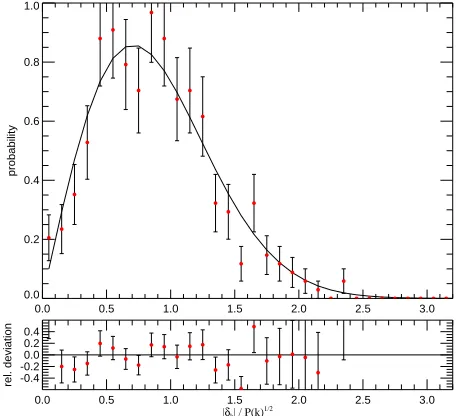
Figure 10: Measured distribution of mode

ampli-tudes in the Millennium Simulation at redshift z=

4.9. Only modes in the k-range 0.03 h/Mpc<k<

0.07 h/Mpc are included (in total 341 modes), with

their amplitude normalised to the square root of the expected linear power spectrum at that redshift. The distribution of modes follows the expected Rayleigh distribution very well. The bottom panel shows the relative deviations of the measurements from this distribution, which are in line with the expected sta-tistical scatter.

(due to growing variations in the volume of domains as a result of our work-load balancing strategy, the PM memory requirements increase somewhat with time). Note that the memory for tree and PM com-putations is not needed concurrently, and this made the simulation feasible. The peak memory consump-tion per processor reached 1850 MB at the end of our simulation, rather close to the maximum possible of 1900 MB.

On the fly analysis. With a simulation of the

size of the Millennium Run, any non-trivial

anal-ysis step is demanding. For example, measuring

the dark matter mass power spectrum over the full dynamic range of the simulation volume would

re-quire a 3D FFT with ∼105 cells per dimension,

which is unfeasible at present. In order to circum-vent this problem, we employed a two stage

pro-“large-scale” and a “small-scale” measurement were combined. The former was computed with a Fourier transform of the whole simulation box, while the latter was constructed by folding the density field

back onto itself13, assuming periodicity for a

frac-tion of the box. The self-folding procedure leads to a sparser sampling of Fourier space on small scales, but since the number of modes there is large, an accurate small-scale measurement is still achieved. Since the PM-step of the simulation code already computes an FFT of the whole density field, we took advantage of this and embedded a measurement of the power spectrum directly into the code. The self-folded spectrum was computed for a 32 times smaller

periodic box-size, also using a 25603 _{mesh, so that}

the power spectrum measurement effectively

corre-sponded to a 819203 mesh. We have carried out a

measurement each time a simulation snapshot was generated and saved on disk. In Figure 9, we show the resulting time evolution of the dark matter power spectrum in the Millennium Simulation. On large scales and at early times, the mode amplitudes grow linearly, roughly in proportion to the cosmological

expansion factor. Nonlinear evolution accelerates

the growth on small scales when the dimensionless

power∆2(k) =k3P(k)/(2π2)approaches unity; this

regime can only be studied accurately using numer-ical simulations. In the Millennium Simulation, we are able to determine the nonlinear power spectrum over a larger range of scales than was possible in

earlier work13, almost five orders of magnitude in

wavenumber k.

On the largest scales, the periodic simulation volume encompasses only a relatively small number of modes and, as a result of the Rayleigh amplitude sampling that we used, these (linear) scales show substantial random fluctuations around the mean

ex-pected power. This also explains why the mean

power in the k-range 0.03 h/Mpc<k<0.07 h/Mpc

lies below the linear input power. In Figure 10,

we show the actual distribution of normalised mode

amplitudes,p|δk|2/P(k), measured directly for this

range of wavevectors in the Millennium Simulation

at redshift z=4.9. We see that the distribution of

mode amplitudes is perfectly consistent with the ex-pected underlying Rayleigh distribution.