Simplex Algorithm for Countable-state Discounted Markov
Decision Processes
∗Ilbin Lee Marina A. Epelman H. Edwin Romeijn Robert L. Smith
November 16, 2014
Abstract
We consider discounted Markov Decision Processes (MDPs) with countably-infinite state spaces, finite action spaces, and unbounded rewards. Typical examples of such MDPs are inventory management and queueing control problems in which there is no specific limit on the size of inventory or queue. Existing solution methods obtain a sequence of policies that converges to optimality in value but may not improve monotonically, i.e., a policy in the sequence may be worse than preceding policies. Our proposed approach considers countably-infinite linear programming (CILP) formulations of the MDPs (a CILP is defined as a linear program (LP) with countably-infinite numbers of variables and constraints). Under standard assumptions for analyzing MDPs with countably-infinite state spaces and unbounded rewards, we extend the major theoretical extreme point and duality results to the resulting CILPs. Under an additional technical assumption which is satisfied by several applications of interest, we present a simplex-type algorithm that is implementable in the sense that each of its iterations requires only a finite amount of data and computation. We show that the algorithm finds a sequence of policies which improves monotonically and converges to optimality in value. Unlike existing simplex-type algorithms for CILPs, our proposed algorithm solves a class of CILPs in which each constraint may contain an infinite number of variables and each variable may appear in an infinite number of constraints. A numerical illustration for inventory management problems is also presented.
1
Introduction
The class of Markov decision processes (MDPs) provides a popular framework which covers a wide variety of sequential decision-making problems. An MDP is classified by its criterion being optimized, its state and action space, whether the problem data is stationary, etc., and those different settings are mostly motivated by applications. For example, in inventory management and queueing control, often times there is no specific limit on the size of inventory or queue, and such problems can be modeled by MDPs with countable state space.
We consider MDPs whose objective is to maximize expected total discounted reward, and that have a countable state space, a finite action space, and unbounded immediate rewards. Specifically, consider a dynamic system that evolves over discrete time periods. In time periods n = 0,1, . . ., a decision-maker observes the current state of the system s ∈ S, where the set of states S is countably-infinite. The decision-maker then chooses an action a∈ A, where the action set A is a finite set. Given that action a is taken in state s, the system makes a transition to a next state
∗
t ∈ S with probability p(t|s, a) and reward r(s, a, t) is obtained. Let r(s, a) denote the expected reward incurred by choosing action a at state s, i.e., r(s, a) =P
t∈Sp(t|s, a)r(s, a, t). A policy is
defined as a decision rule that dictates which action to execute and the rule may in general be conditioned on current state, time, and the whole history of visited states and actions taken. The goal is to find a policy that maximizes the expected total discounted reward, with discount factor
α ∈(0,1), over the infinite-horizon for any starting state. In this paper, we refer to this problem as a countable-state MDP for short.
For a policyπ,Vπ(s) denotes the expected total discounted reward obtained by executingπstarting from state s, and we call Vπ the value function of policy π. For s ∈ S, let V?(s) denote the supremum of Vπ(s) over all policiesπ; thenV? is the optimal value function. Thus, the goal of the MDP problem can be rephrased as finding a policy whose value function coincides with the optimal value function. For more precise definitions, see Section 2.1.
1.1 Motivation and Contribution
Countable-state MDPs were studied by many researchers, including [4, 10, 12, 21, 22, 23], with predominant solution methods summarized as the three algorithms in [21, 22] and [23]. We will review these in Section 1.2 in detail. Each of the three algorithms computes a sequence of real-valued functions onS that converges to the optimal value function V?. Also, for the algorithms in [21] and [23], methods to obtain a sequence of policies whose value functions converge pointwise to the optimal value function were provided as well. However, the value function of policies obtained by these two methods may not improve in every iteration. In other words, a policy obtained in a later iteration may be worse (for some starting states) than a previously obtained policy. In practice, one can run those algorithms only for a finite time, obtaining a finite sequence of policies. Upon termination, it should be determined which policy to execute. Without monotonicity of value functions of obtained policies, the value functions of those policies should be exactly computed in order to find the best one. However, computing the value function of even one policy takes an infinite amount of computation for countable-state MDPs, and even if the policies are evaluated approximately, it still requires a considerable amount of computation (in addition to the running time of the algorithm). On the other hand, if the sequence of value functions of obtained policies is guaranteed to be monotone, then the last obtained policy is always guaranteed to be the best one so far. The key motivation of this paper is to develop an algorithm that finds a sequence of policies whose value functions improve in every iteration and converge to the optimal value function. We propose an algorithm that has both of the characteristics under the assumptions considered in [12] to analyze countable-state MDPs with unbounded rewards (introduced in Section 2.1) and an additional technical assumption (introduced at the end of Section 4.1), which are satisfied by application examples of interest as we show in this paper.
For countable-state MDPs, the equivalent LP formulations have a countably-infinite number of variables and a countably-infinite number of constraints. Such LPs are called countably-infinite linear programs (CILPs). General CILPs are challenging to analyze or solve mainly because useful theoretical properties of finite LPs (such as duality) fail to extend to general CILPs. We sum-marize the challenges for general CILPs in Section 1.2. Due to these hurdles, there are only a few algorithmic approaches to CILPs in the literature ([7, 8, 19]) (all of these are simplex-type algorithms, i.e., they navigate through extreme points of the feasible region). In particular, for a CILP formulation of non-stationary MDPs with finite state space, which can be considered to be a subclass of countable-state MDPs, [8] recently provided duality results, characterization of extreme points, and an implementable simplex algorithm that improves in every iteration and converges to optimality.
However, classes of CILPs considered so far ([7, 8, 19]) have a special structure that each constraint has only a finite number of variables and each variable appears only in a finite number of constraints. In the CILP formulation of countable-state MDPs we present in Section 3, each constraint may have an infinite number of variables and each variable may appear in an infinite number of constraints (i.e., the coefficient matrix of the CILP can be “dense”) as we illustrate by Example 2. Another key contribution of this paper is that we show that even without restrictions on positions of nonzeros in the coefficient matrix, the dynamic programming structure in the coefficient matrix of the CILP formulation of countable-state MDPs still enables us to establish the standard LP results and develop a simplex-type algorithm.
1.2 Literature Review
In this section, we first review the existing solution methods for countable-state MDPs as discussed in [21, 22, 23].
The algorithm suggested in [23] is an extension of value iteration to countable-state MDPs. In general, value iteration computes a sequence of real-valued functions on S that converges to the optimal value function. To remind the readers, value iteration for finite-state MDPs starts with a function V0 :S →R and for k = 1,2, . . ., computes a function Vk :S →R in iteration k by the following recursion formula:
Vk(s),max a∈A
(
r(s, a) +αX
t∈S
p(t|s, a)Vk−1(t)
)
for s∈ S. (1)
Extending this to countable-state MDPs requires an adjustment in order for each iteration to finish in finite time. The value iteration for countable-state MDPs first selects a function u:S →R and then, in iteration k, computes Vk(s) by (1) only for s ≤ k and lets Vk(s) = u(s) for s > k. In [23], it was shown that Vk converges pointwise to the optimal value functionV? and error bounds on the approximations were provided. In iteration k, a policy πk :S → A (i.e., a stationary and deterministic policy) is obtained by assigning the action that achieves the maximum in (1) tos≤k
and an arbitrary action tos > k. It was also shown in [23] thatVπk converges pointwise toV? but
the convergence may not be monotone.
1. ObtainVk:S →R that satisfies
Vk(s) =r(s, πk−1(s)) +αX
t∈S
p(t|s, πk−1(s))Vk(t) for s∈ S; (2)
2. Choose πk:S → Athat satisfies
πk(s)∈arg max a∈A
(
r(s, a) +αX
t∈S
p(t|s, a)Vk(t)
)
fors∈ S. (3)
Each iteration consists of computing the value function of the current (stationary and deterministic) policy (Step 1) and obtaining a new policy based on the evaluation (Step 2). The extension of policy iteration to countable state space is as follows: after selecting a function u :S → R, in iteration k, it computes Vk that satisfies (2) for s≤k and Vk(s) = u(s) for s > k, and then finds πk that satisfies (3) only for s≤k. It was shown in [21] thatVk obtained by this method also converges pointwise to V? and error bounds on the approximations were provided. One can extendπk to the entire state space S by assigning an arbitrary action tos > k; thenVπk converges pointwise to V?
but again, the convergence may not be monotone.
Another method, proposed in [22], is to solve successively larger but finite-state approximations of the original MDP to optimality. The real-valued functions onS obtained by this method were also proven to converge pointwise toV?. A sequence of policies covering S is also obtained by this algorithm in a similar manner but pointwise convergence of their value functions was not established in the paper.
It should be pointed out that the above three papers only considered the case where the reward function is uniformly bounded. However, in the aforementioned applications of countable-state MDPs, immediate reward typically goes to infinity as the inventory level or the number of cus-tomers in queue goes to infinity, which suggests the need to consider countable-state MDPs with unbounded immediate reward functions. For brevity, let us refer to a set of assumptions on transi-tion probabilities and rewards as a setting in the following literature review. Under three different settings with unbounded rewards, [9, 11, 20] studied properties of countable-state MDPs. In [24], each of the three settings with unbounded rewards in [9, 11, 20] was equivalently transformed into a bounded one. Therefore, the algorithms and results mentioned in previous paragraphs for bounded case were extended to the three unbounded problems in [9, 11, 20]. Meanwhile, [4] extensively reviewed conditions under which the extension of the value iteration in [23] converges to optimality in value and studied its rate of convergence. The setting in [4] is more general than the settings in [9, 11, 20] but one cannot check whether it holds for given transition probabilities and rewards without solving the MDP since it includes an assumption on the optimal value function. In this paper, we consider the setting in [12] (Section 6.10) for countable-state MDPs with unbounded rewards (Assumptions A1, A2, and A3 in Section 2.1 of this paper). One can easily show that this setting covers the three settings in [9, 11, 20]; it is a special case of the one in [4] but it is checkable for given parameters without solving the MDP and has enough generality to cover many applications of interest.
(for more details, see [7, 8]). First, there is an example in which a CILP and its dual have a duality gap ([15]). Also, there is a CILP that has an optimal solution but does not have an extreme point optimal solution ([3]). Even for CILPs that have an extreme point optimal solution, extending the simplex method is challenging. A pivot operation may require infinite computation, and hence not be implementable ([3, 19]). Moreover, [7] provided an example of a CILP in which a strictly improving sequence of extreme points may not converge in value to optimality, which indicates that proving convergence to optimality requires careful considerations. However, some of LP results can be extended by considering more structured CILPs ([8, 14, 15]) or finding appropriate sequence spaces ([6]).
1.3 Organization
The rest of this paper is organized as follows. In Section 2, we formally define countable-state MDPs, introduce assumptions on problem parameters, give two application examples, and review some results established in literature. In Section 3, we introduce primal and dual CILP formula-tions for countable-state MDPs, prove strong duality, define complementary slackness, and prove the equivalence of complementary slackness and optimality. Then, in Section 4, we introduce an implementable simplex-type algorithm solving the dual CILP. We show that the algorithm obtains a sequence of policies whose value functions strictly improve in every iteration and converge to the optimal value function. Section 5 illustrates computational behavior of the algorithm for inventory management problem instances and Section 6 concludes the paper with discussion and some future research directions.
2
Countable-State MDP
2.1 Problem Formulation
We continue to use the notation introduced in the previous section: countably-infinite state setS, finite action setA, transition probabilities p(t|s, a) and immediate rewardr(s, a, t) (along with the expected immediate reward r(s, a)) fors, t∈ S and a∈ A, and discount factor 0< α <1. We let S ={1,2, . . .} and A={1,2, . . . , A} unless otherwise specified.
A policyπ is a sequenceπ={π1, π2, . . .}of probability distributionsπn(·|hn) over the action setA, wherehn= (s0, a0, s1, a2, . . . , an−1, sn) is the whole observed history at the beginning of period n. A policy π is called Markov if the distributionsπn depend only on the current state and time, i.e.,
πn(·|hn) = πn(·|sn). A Markov policy π is called stationary if the distributions πn do not depend on time n, i.e., πn(·|s) = πm(·|s) for all s ∈ S and time periods m and n. A policy π is said to be deterministic if each distribution πn(·|hn) is concentrated on one action. For a stationary and deterministic policyπand a states,π(s) denotes the action chosen byπats. Let Π,ΠM,ΠM D,ΠS, and ΠSD denote the set of all policies, Markov policies, Markov deterministic policies, stationary policies, and stationary deterministic policies, respectively.
Given an initial state distribution β, each policy π induces a probability distribution Pπβ on se-quences{(sn, an)}∞n=0, where (sn, an)∈ S × Aforn= 0,1, . . ., and defines a state process{Sn}∞n=0
and an action process {An}∞n=0. We denote by E
β
expected total discounted reward of a policyπ with initial state distribution β is defined as
Vπ(β),Eπβ
"∞ X
n=0
αnr(Sn, An)
#
. (4)
We call Vπ(β) the value of policy π with initial state distribution β, or simply the value of policy
π whenever it is clear which initial state distribution is used. For those initial state distributions concentrated on one state s, we use a slight abuse of notation in (4): Vπ(s) where β(s) = 1 for a states. Vπ :S →Ris called the value function of policyπ.
A policyπ? is said to beoptimal for initial state distribution β ifVπ?(β) =V?(β),supπ∈ΠVπ(β).
A policy π? is said to be optimal for initial state s if Vπ?(s) = V?(s) , supπ∈ΠVπ(s). We call
V? :S →Rthe optimal value function of the MDP or simplythe optimal value function. A policy
π? is defined to be optimal ifVπ?(s) =V?(s) for all s∈ S, i.e., if it is optimal for any initial state.
The goal of the decision maker is to find an optimal policy.
Let us define additional notation that will come in handy in the rest of the paper. Given a policyπ and states s, t∈ S,Pπn(t|s) denotes the probability of reaching statet after ntransitions starting from stateswhen policy π is applied, with Pπ0(t|s),1{t=s}. Pπn denotes the transition probability matrix of policy π for n transitions with both rows and columns indexed by states.
Pπ0, defined similarly, is denoted asI. For simplicity, we denotePπ1(t|s) andPπ1 as Pπ(t|s) andPπ, respectively. For a stationary policy σ (in this paper, notationσ is used to emphasize the choice of a stationary policy) and a state s∈ S,rσ(s) denotesr(s, σ(s)), the expected immediate reward atswhen σ is applied, andrσ denotes the reward vector indexed by states.
Throughout the paper, we will make the following assumptions, which enable us to analyze countable-state MDPs with unbounded rewards:
Assumption (cf. Assumptions 6.10.1 and 6.10.2 of [12]) There exists a positive real-valued functionw on S satisfying the following:
A1 |r(s, a)| ≤w(s) for all a∈ A ands∈ S;
A2 There exists κ, 0≤κ <∞, for which
∞
X
t=1
p(t|s, a)w(t)≤κw(s)
for alla∈ Aand s∈ S;
A3 There exists λ, 0≤λ <1, and a positive integer J such that
αJ ∞
X
t=1
PπJ(t|s)w(t)≤λw(s)
for allπ ∈ΠM D.
Assumption 1 tells us that the absolute value of the reward function is bounded by the function
w. In other words, the function w provides a “scale” of reward that can be obtained in each state. Assumption 2 can be interpreted as that the transition probabilities prevent the expected scale of immediate reward after one transition from being larger than the scale in the current state (multiplied byκ). Assumption 3 can be interpreted similarly, but forJ transitions. However, note thatλis strictly less than one, which is important because λwill play a role similar to that of the discount factor α in our following analysis.
2.2 Examples
We give two examples of countable-state MDPs with unbounded costs that satisfy Assumptions A1, A2, and A3.
Example 1 (Example 6.10.2 in [12])Consider an infinite-horizon inventory management prob-lem with a single product and unlimited inventory capacity where the objective is to maximize the expected total discounted profit. LetS ={0,1, . . .},A={0,1, . . . , M}, and
p(t|s, a) =
0 t > s+a ps+a−t s+a≥t >0
qs+a t= 0,
wherepkdenotes the probability of demand ofkunits in any period, andqk =P∞j=kpj denotes the probability of demand of at leastk units in any period. Fors∈ S and a∈ A, the reward r(s, a) is given as
r(s, a) =F(s+a)−O(a)−h·(s+a),
where
F(s+a) = s+a−1
X
j=0
bjpj+b(s+a)qs+a,
withb >0 representing the per-unit price,O(a) =K+cafora >0 andO(0) = 0 representing the ordering cost, and h > 0 representing the cost of storing one unit of product for one period. It is reasonable to assume P∞
k=0kpk<∞, i.e., the expected demand is finite. Then,
|r(s, a)| ≤b(s+M) +K+cM +h(s+M) =K+M(b+c+h) + (b+h)s,C+Ds
by lettingC,K+M(b+c+h) andD,b+h. Letw(s),C+Dsso that A1 holds. Since
∞
X
t=0
p(t|s, a)w(t) = s+a
X
t=1
ps+a−t·w(t) +qs+a·w(0) = s+a−1
X
t=0
pt·w(s+a−t) +qs+a·w(0)
=C+D
s+a−1 X
t=0
(s+a−t)pt≤C+D(s+a)≤w(s) +DM,
by Proposition 6.10.5(a) in [12], A2 and A3 are also satisfied.
soS ={0,1, . . .}. LetA1 andA2be finite sets of nonnegative numbers and letA=A1× A2. If the
decision-maker chooses (a1, a2)∈ A1× A2 in a period, then the number of arrivals in the period is
a Poisson random variable with meana1 and the number of served (thus, leaving) customers in the period is the minimum of a Poisson random variable with mean a2 and the number of customers in the system at the beginning of the period plus the number of arrivals in the period. (That is, we assume that order of the events in a period is: the decision-maker observes the current state and chooses two numbersa1∈ A1 and a2∈ A2, arrivals occur, and then services are provided and
served customers leave.) Fors∈ S, a= (a1, a2)∈ A, the immediate reward is
r(s, a) =−cs−d1(a1)−d2(a2),
wherecis a positive constant,d1(·) is the flow control cost function, andd2(·) is the service control cost function. The reward is linear ins, which is justified by the well-known Little’s Law.
In the flow and service control problem in [2], it was assumed that in a period, at most one customer arrives and at most one customer leaves the system, which no longer holds in this example.
Let C , c and D , maxa1∈A1|d1(a1)|+ maxa2∈A2|d2(a2)|. Then A1 is satisfied with w(s) ,
Cs+D.
In addition,
X
t∈S
p(t|s, a)w(t) =D+C ∞
X
t=0
p(t|s, a)t=D+C
"s−1 X
t=0
p(t|s, a)t+
∞
X
u=0
p(s+u|s, a)(s+u)
#
≤D+Cs+
∞
X
u=0
p(s+u|s, a)u≤w(s) +
∞
X
u=0
e−a1max(a1
max)u
u! u=w(s) +Ca
1 max,
where the second inequality is obtained by considering maximum arrival rate a1max = maxA1 and
zero service rate. Therefore, by Proposition 6.10.5(a) in [12], A2 and A3 are satisfied.
Parts (b) and (c) of Proposition 6.10.5 in [12] provide two other sufficient conditions to satisfy A2 and A3.
2.3 Background
We conclude this section by reviewing some technical preliminaries that were established in the literature and will be used in this paper.
By the following theorem, we can limit our attention to policies that are stationary and determin-istic.
Theorem 2.1 (cf. Theorem 6.10.4 of [12]) Countable-state MDPs under Assumptions A1, A2, and A3 satisfy the following.
(1) There exists an optimal policy that is stationary and deterministic. (2) The optimal value function V? is the unique solution of
y(s) = max a∈A
(
r(s, a) +α ∞
X
t=1
p(t|s, a)y(t)
)
for s∈ S.
In particular, for any stationary deterministic policy σ, Vσ equals the optimal value function of a new MDP obtained by allowing only one action σ(s) fors∈ S, and thus, Vσ is the unique solution of
y(s) =r(s, σ(s)) +α ∞
X
t=1
p(t|s, σ(s))y(t) for s∈ S,
or y=rσ+αPσy in the infinite vector and matrix notation.
Define
L,
( J
1−λ ifακ= 1
1 1−λ
1−(ακ)J
1−(ακ) otherwise.
It has been shown that the value function of any Markov policy is bounded by Lw:
Proposition 2.2 (cf. Proposition 6.10.1 of [12]) If Assumptions A1, A2, and A3 are satisfied,
|Vπ(s)| ≤Lw(s) for anys∈ S and π∈ΠM. (5)
In the rest of this subsection, we review some real analysis results that will be used in this paper for exchanging two infinite sums, an infinite sum and an expectation, or a limit and an expecta-tion.
Proposition 2.3 (cf. Tonelli’s theorem on page 309 of [17]) Given a double sequence {aij} for i= 1,2, . . .,j = 1,2, . . ., if aij ≥0 for all iand j, then
∞
X
i=1 ∞
X
j=1
aij =
∞
X
j=1 ∞
X
i=1
aij.
Proposition 2.4 (Theorem 8.3 in [18]) Given a double sequence {aij} for i = 1,2, . . ., j = 1,2, . . ., if P∞
i=1 P∞
j=1|aij|converges, then
∞
X
i=1 ∞
X
j=1
aij =
∞
X
j=1 ∞
X
i=1
aij <∞.
This proposition is a special case of Fubini-Tonelli theorem, which is obtained by combining Fubini’s theorem (see Theorem 19 on page 307 of [17]) and Tonelli’s theorem. We will also use the following special case of monotone convergence theorem (MCT).
Proposition 2.5 (Series version of monotone convergence theorem, Corollary 5.3.1 of [13])
If Xi are nonnegative random variables fori= 1,2, . . ., then
E
"∞ X
i=1
Xi
#
=
∞
X
i=1
E[Xi].
Proposition 2.6 (Dominated convergence theorem, Theorem 5.3.3 of [13]) If a sequence of random variables {Xi}∞i=1 converges to a random variable X and there exists a dominating
random variable Z such that |Xi| ≤Z for i= 1,2, . . . and E[|Z|]<∞, then
3
CILP Formulations
In this section, we introduce primal and dual CILP formulations of countable-state discounted MDPs. We start with a straightforward result which was used in [12] and [16] without being explicitly stated.
Lemma 3.1 A policy is optimal if and only if it is optimal for an initial state distribution that has a positive probability at every state.
Proof: For a policyπ and an initial state distributionβ, observe that
Vπ(β) =Eπβ
" ∞ X
n=0
αnr(Sn, An)
#
=
∞
X
s=1
β(s)Esπ
"∞ X
n=0
αnr(Sn, An)
#
=
∞
X
s=1
β(s)Vπ(s).
Since Vπ(s)≤V?(s) for any s∈ S, and β(s)>0 for anys∈ S, a policy π maximizesVπ(β) if and only if it maximizes Vπ(s) for each state s, and thus, the equivalency is proven.
Using this lemma, we equivalently consider finding an optimal policy for a fixed initial state distri-bution that satisfies
β(s)>0 for alls∈ S. (6)
Additionally, we require thatβ satisfies
βTw=
∞
X
s=1
β(s)w(s)<∞. (7)
(7) will help us show that a variety of infinite series we consider in this paper converge. Note that
β is not a given problem parameter and that there are many functional forms ofwthat allow us to choose β satisfying (6) and (7). For example, if w∈ O(sm) for some positive numberm (in other words, w is asymptotically dominated by a polynomial in s), then we can easily find β satisfying the conditions by modifying an exponential function appropriately.
Now we introduce a CILP formulation of a countable-state MDP. Let kykw , sups∈S |y(s)|
w(s) for
y∈R∞ and Yw,{y∈R∞:kykw <∞}. Consider the following CILP:
(P) min g(y) =
∞
X
s=1
β(s)y(s) (8)
s.t. y(s)−α ∞
X
t=1
p(t|s, a)y(t)≥r(s, a) for s∈ S and a∈ A (9)
y∈Yw. (10)
A CILP formulation consisting of (8) and (9) was introduced in Chapter 2.5 of [16] for MDPs with uniformly bounded rewards. By adding constraint (10), one can apply essentially the same arguments to countable-state MDPs being considered in this paper (i.e., ones with unbounded rewards but satisfying Assumptions A1, A2, and A3) to show that the optimal value function
MDPs a special case. However, assumptions used in the latter are quite different from ours and it is not known either if his set of assumptions implies ours or vice versa.)
A few remarks about (P) are in order. Note that for any y ∈ Yw, the objective function value is always finite because of (7). Also, the infinite sum in each constraint, P∞
t=1p(t|s, a)y(t) for
s ∈ S and a ∈ A, can be shown to be finite for any y ∈ Yw by using Assumption A2. Also, under Assumptions A1, A2, and A3, value functions of all Markov policies belong to Yw due to Proposition 2.2, so (10) does not exclude any solution of interest. Since, for any optimal policy
π?,
V?(β) =Vπ?(β) =
∞
X
s=1
β(s)Vπ?(s) =
∞
X
s=1
β(s)V?(s), (11)
the optimal value of (P) equalsV?(β). Lastly, we note thatYwis a Banach space, so (P) is a problem of minimization of a linear function in a Banach space while satisfying linear inequalities.
We also consider the following CILP formulation of a countable-state MDP:
(D) maxf(x) =
∞
X
s=1
A
X
a=1
r(s, a)x(s, a) (12)
s.t. A
X
a=1
x(s, a)−α ∞
X
t=1
A
X
a=1
p(s|t, a)x(t, a) =β(s) for s∈ S (13)
x≥0, x∈l1,
where l1 is the space of absolutely summable sequences: x ∈ l1 means P∞s=1PAa=1|x(s, a)| <
∞.
Derivations of (D) can be found in the literature even for more general classes of MDPs (e.g., see Chapter 8 of [2] or Chapter 12 of [5]). However, we provide a high-level derivation of (D) in Appendix A, in part because it also gives a proof of strong duality between (P) and (D) (Theo-rem 3.3); due to this relationship, we will refer to (P) as the primal problem, and (D) — as the dual problem. Briefly, (D) is derived by a convex analytic approach which considers the MDP as a convex optimization problem maximizing a linear functional over the convex set of occupancy measures. (An occupancy measure corresponding to a policy is the total expected discounted time spent in different state-action pairs under the policy; for a precise definition, see Appendix A.) It is well known that F, which denotes the set of feasible solutions to (D), coincides with the set of occupancy measures of stationary policies. For any stationary policyσ and its occupancy measure
x ∈ F, Vσ(β) is equal to the objective function value of (D) at x. An optimal stationary policy (which is known to be an optimal policy) can therefore be obtained from an optimal solution to (D) by computing the corresponding stationary policy (for more details, see Appendix A).
The following visualization of constraint (13) will help readers understand the structure of (D). Using infinite matrix and vector notation, constraint (13) can be written as
[M1|M2|. . .|Ms|. . .]x=β. (14)
Here, fors∈ S,Msis an∞×Amatrix whose rows are indexed by states andMs=Es−αPs, where each column of Es is the unit vector es, and the ath column of Ps is the probability distribution
p(·|s, a).1
1Note that the rows ofPs are indexed by next states. Meanwhile, given a stationary deterministic policyσ, the
Remark 3.2 Let us re-visit Example 2. For any state s, for any action a = (a1, a2) such that
a1 >0, transition to any state t≥shas a positive probability. That is, the ath column of Ps has an infinite number of positive entries. On the other hand, any statescan be reached by a transition from any state t≥s by an action a= (a1, a2) such that a2 >0. That is, for any t≥s, the entry of Pt at the sth row and the ath column is positive. Consequently, in the CILP (D) for Example 2, there are variables that appear in an infinite number of constraints (unless A1 ={0}) and each
constraint has an infinite number of variables (unless A2={0}).
The following strong duality theorem is proven in Appendix A.
Theorem 3.3 Strong duality holds between (P) and (D), i.e.,g(y∗) =f(x∗), where y∗ and x∗ are optimal solutions of (P) and (D), respectively.
Note that (D) has only equality constraints and non-negativity constraints, and thus can be said to be in standard form. The main goal of this paper is to develop a simplex-type algorithm that solves (D). A simplex-type algorithm is expected to move along an edge between two adjacent extreme points, improving the objective function value at every iteration, and converge to an extreme point optimal solution. The following characterization of extreme points of F is also well known in literature (e.g., Theorem 11.3 of [5]).
Theorem 3.4 A feasible solution x of (D) is an extreme point of F if and only if for any s∈ S, there exists a(s)∈ Asuch that x(s, a(s))>0 and x(s, b) = 0 for allb6=a(s). That is, the extreme points of F correspond to stationary deterministic policies.
Therefore, it is natural to define basic feasible solution in the following way.
Definition 3.5 A feasible solution x to (D) is defined to be a basic feasible solution of (D) if for anys∈ S, there exists a(s)∈ A such thatx(s, a(s))>0 and x(s, b) = 0 for allb6=a(s).
Note that a basic feasible solution is determined by choosing one column from each block matrix
Ms in (14) for s ∈ S. For a basic feasible solution x and for s∈ S, the unique action a(s) that satisfiesx(s, a(s))>0 is called a basic action ofx at states. Basic actions of x naturally define a stationary deterministic policy, say,σ. Recall thatF is the set of occupancy measures of stationary policies; moreover, the set of extreme points ofF coincides with the set of occupancy measures of stationary deterministic policies. Thus, conversely, the extreme pointx is the occupancy measure of the stationary deterministic policyσ.
The next theorem follows immediately, based on the existence of an optimal policy that is stationary and deterministic and the correspondence between stationary deterministic policies and extreme points (Theorem 11.3 of [5]).
Theorem 3.6 (D) has an extreme point optimal solution.
Next, we define complementary slackness between solutions of (P) and (D), and prove its equivalence to optimality.
Definition 3.7 (Complementary slackness)Supposex∈ F andy∈Yw. xandyare said to satisfy complementary slackness(or be complementary) if
x(s, a)
"
r(s, a)− y(s)−α ∞
X
t=1
p(t|s, a)y(t)
!#
= 0 for all s∈ S, a∈ A. (15)
respectively.
Proof: In Appendix B.
Theorem 3.9 (Complementary slackness necessity) If y and x are optimal to (P) and (D), re-spectively, then they are complementary.
Proof: In Appendix C.
Given a basic feasible solution x, let σ be the corresponding stationary deterministic policy. By Theorem 2.1(2) and the definition of complementary slackness, ay ∈Yw is complementary with x if and only if y is the value function of σ. Since the value function of a policy is unique, for any basic feasible solutionx, there exists a uniquey ∈Yw that is complementary withx, and moreover,
y satisfies|y| ≤Lw by Proposition 2.2.
Recently in [6], it was shown that for general CILPs, weak duality and complementary slackness could be established by choosing appropriate sequence spaces for primal and dual, and the result was applied to CILP formulations of countable-state MDPs with bounded rewards. In the paper, one of the conditions for the choice of sequence space is that the objective function should converge for any sequence in the sequence space. However, in (D), the sequence spacel1 does not guarantee
convergence of the objective function (but the objective function converges for any feasible solution of (D) as shown in Appendix A). Thus, for countable-state MDPs with unbounded rewards being considered in this paper, applying the choice of sequence spaces in [6] would yield a different CILP formulation from (D), in which the feasible region may not coincide the set of occupancy measures of stationary policies.
We conclude this section with the next lemma which will be useful in later sections.
Lemma 3.10 Any x∈ F satisfies
∞
X
s=1
A
X
a=1
x(s, a) = 1 1−α.
Proof: In Appendix D.
4
Simplex Algorithm
costs of only a finite number of nonbasic variables using only finite computation and data in every iteration. We should also ensure that the algorithm improves in every iteration and converges to optimality despite the above restrictions.
In [8], a simplex algorithm for non-stationary MDPs with finite state space that satisfies all of the requirements was introduced. Here we introduce a simplex algorithm that satisfies all of the requirements for a larger class of MDPs, namely, countable-state MDPs.
4.1 Approximating Reduced Costs
In this section we describe how we approximate reduced costs and prove an error bound for the approximation. Let x be a basic feasible solution to (D) and let y ∈ Y be its complementary solution. We first define reduced costs.
Definition 4.1 Given a basic feasible solution xand the corresponding complementary solutiony, reduced cost γ(s, a) of state-action pair (s, a) ∈ S × A is defined as negative of the slack in the corresponding constraint in (P):
γ(s, a),r(s, a) +α ∞
X
t=1
p(t|s, a)y(t)−y(s). (16)
For a state-action pair (s, a) such that x(s, a) >0, the reduced cost γ(s, a) is zero by complemen-tarity. Ifγ(s, a)≤0 for all (s, a)∈ S × A, it means thaty is feasible to (P), and thus, xis optimal to (D) by Theorem 3.8.
Letσbe the stationary deterministic policy corresponding tox. Fix a statesand an actiona6=σ(s) and consider a stationary deterministic policy τ obtained from σ by changing the basic action at state sto a. We call this procedure for obtaining τ from σ a pivot operation. Letz be the basic feasible solution corresponding to τ. The next proposition shows the relation between the change in objective function value made by this pivot operation and the reduced costγ(s, a).
Proposition 4.2 In the aforementioned pivot operation, the difference in objective function values of x and z is given by
f(z)−f(x) =γ(s, a)
∞
X
t=1
β(t)
∞
X
n=0
αnPτn(s|t).
If the reduced cost γ(s, a) is positive, then the objective function strictly increases after the pivot operation, by at least β(s)γ(s, a).
Proof: First, note that we can easily show that the infinite sum on the right hand side is finite because probabilities are less than or equal to one. Letyandvbe the complementary solutions ofx
andz, respectively. Then, we havey=rσ+αPσyandv=rτ+αPτv. Thus,v−y=rτ+αPτv−y=
rτ +αPτ(v−y) +αPτy−y where the last equality follows because each entry of Pτv and Pτy is finite (since |v|and |y|are bounded byLw and each entry ofPτwis finite by Assumption A2). By Theorem C.2 in [12], (I−αPτ)−1 exists for any stationary policyτ and we have2
(I −αPτ)−1 ,I+αPτ +α2Pτ2+. . . .
2
BecauseαPτ is a bounded linear operator onYw equipped with the normk · kw and the spectral radius ofαPτ
Therefore, we havev−y= (I−αPτ)−1(rτ+αPτy−y). Entries of the infinite vectorrτ+αPτy−y are
(rτ +αPτy−y)(t) =r(t, τ(t)) +α
∞
X
t0=1
p(t0|t, τ(t))y(t0)−y(t) =
(
γ(s, a) ift=s
0 otherwise.
Therefore,
f(z)−f(x) =βTv−βTy=βT(v−y) =βT(I−αPτ)−1(rτ+αPτy−y)
=γ(s, a)
∞
X
t=1
β(t)
∞
X
n=0
αnPτn(s|t),
establishing the first result. Because
∞
X
t=1
β(t)
∞
X
n=0
αnPτn(s|t)≥β(s)Pτ0(s|s) =β(s)>0,
the second claim is also proven.
Computing the reduced cost of even one state-action pair requires computing y. Recall that y is the value function of the policy σ. Computingy requires an infinite amount of computation and an infinite amount of data, no matter how it is computed, either by computing the infinite sum (4) or solving the infinite system of equationsy=rσ+αPσy.
For a given policy σ, we consider approximating the complementary solution y by solving the followingN-state truncation of the infinite system of equationsy=rσ+αPσy. LetN be a positive integer. The approximate complementary solution, which we denote as yN, is defined to be the solution of the following finite system of equations:
yN(s) =rσ(s) +α N
X
t=1
Pσ(t|s)yN(t) for s= 1, . . . , N. (17)
Note thatyN is the value function of policyσ for a new MDP obtained by replacing states greater than N by an absorbing state in which no reward is earned, and thus, yN is an approximation of
y obtained from the N-state truncation of the original MDP. The next lemma provides an error bound for the approximate complementary solution.
Lemma 4.3 For any positive integer N, the approximate complementary solution yN satisfies
|yN(s)−y(s)| ≤LX
t>N
∞
X
n=1
αnPσn(t|s)w(t) for s= 1, . . . , N.
The error bound on the right hand side converges to zero as N → ∞. Therefore, yN converges pointwise to y as N → ∞.
Proof: In Appendix E.
Using the approximate complementary solution, we define approximate reduced costs of nonbasic variables that belong to the N-state truncation:
γN(s, a),r(s, a) +α
N
X
t=1
Note that γN(s, a) is an approximation of reduced costγ(s, a) computed by using yN in place of
y. The next lemma provides an error bound on the approximate reduced cost.
Lemma 4.4 For any positive integer N, the approximate reduced cost γN satisfies
|γN(s, a)−γ(s, a)| ≤δ(σ, s, a, N) for s= 1, . . . , N, a∈ A,
where we define
δ(σ, s, a, N),LX
t>N
∞
X
n=1
αnPσn(t|s)w(t)+αL
N
X
t=1
p(t|s, a) X t0>N
∞
X
n=1
αnPσn(t0|t)w(t0)+αLX
t>N
p(t|s, a)w(t).
(19)
Proof: By Lemma 4.3 and (5), for anys≤N and a∈ A,
|γN(s, a)−γ(s, a)| ≤α
N
X
t=1
p(t|s, a)|yN(t)−y(t)|+|yN(s)−y(s)|+αX
t>N
p(t|s, a)|y(t)|
≤αL
N
X
t=1
p(t|s, a) X t0>N
∞
X
n=1
αnPσn(t0|t)w(t0) +LX
t>N
∞
X
n=1
αnPσn(t|s)w(t) +αLX
t>N
p(t|s, a)w(t)
=δ(σ, s, a, N),
which proves the lemma.
By using Assumptions A2 and A3 and arguments similar to those in Appendix E, it is not hard to prove the following proposition aboutδ(σ, s, a, N).
Proposition 4.5 For any positive integer N and for σ∈ΠSD, s= 1, . . . , N, and a∈ A,
δ(σ, s, a, N)≤L(L+ακL+ακ)w(s), (20)
and for any σ ∈ΠSD, s= 1, . . . , N, anda∈ A,
δ(σ, s, a, N)→0 as N → ∞. (21)
Thus, by this proposition and Lemma 4.4, we have γN(s, a) → γ(s, a) as N → ∞ for any state-action pair (s, a).
To design a convergent simplex-like algorithm for solving (D), we need to assume the existence of a uniform (policy independent) upper bound on δ(σ, s, a, N), i.e., ¯δ(s, a, N) ≥δ(σ, s, a, N) for all
σ∈ΠSD, positive integer N,s≤N, and a∈ A, such that
¯
δ(s, a, N)→0 asN → ∞for any (s, a). (22)
4.2 Simplex Algorithm
Our simplex algorithm finds a sequence of stationary deterministic policies whose value functions strictly improve in every iteration and converge to the optimal value function. Let σk denote the stationary deterministic policy our algorithm finds in iterationk. Letxk denote the corresponding basic feasible solution of (D) and yk denote the complementary solution.
The intuition behind the algorithm can be described as follows. Ifσkis not optimal,ykis not feasible to (P), and thus, there is at least one nonbasic variable (state-action pair) whose reduced cost is positive. To identify such a variable with finite computation, in each iteration we considerN-state truncations of the MDP, increasing N as necessary. As N increases, the variable’s approximate reduced cost approaches its exact value, and for sufficiently large N becomes sufficiently large to deduce (by Lemma 4.4) that the (exact) reduced cost of the variable is positive. Moreover, in choosing a variable for the pivot operation, the algorithm selects a nonbasic variable that not only has a positive reduced cost, but also has the largest approximate reduced cost (weighted by
β) among all nonbasic variables in the N-state truncation; this choice is similar to the Dantzig pivoting rule for finite LPs. Choosing a nonbasic variable with a positive reduced cost ensures strict improvement, and choosing one with the largest weighted approximate reduced cost enables us to prove convergence to optimality. (As demonstrated by a counter-example in [7], an arbitrary sequence of improving pivot operations may lead to convergence to a suboptimal value.) A unique feature of our algorithm is that in each iteration it adjusts N, the size of finite-state truncation, dynamically until a condition for performing a pivot operation is satisfied, whereas existing solution methods for countable-state MDPs increase the size by one in every iteration.
An implementable simplex algorithm for countable-state MDPs
1. Initialize: Set iteration counterk= 1. Fix basic actionsσ1(s)∈ Afors∈ S.3
2. Find a nonbasic variable with the most positive approximate reduced cost:
(a) SetN := 1 and setN(k) :=∞.
(b) Compute the approximate complementary solution,yk,N(s) for s= 1, . . . , N by solving (17).
(c) Compute the approximate reduced costs,γk,N(s, a) for s= 1, . . . , N, a∈ Aby (18).
(d) Find the nonbasic variable achieving the largest approximate nonbasic reduced cost weighted by β:
(sk,N, ak,N) = arg max
(s,a)
β(s)γk,N(s, a). (23)
(e) If γk,N(sk,N, ak,N) > ¯δ(sk,N, ak,N, N), set N(k) = N, (sk, ak) = (sk,N, ak,N), and
σk+1(sk) = ak, σk+1(s) = σk(s) for s 6= sk, and go to Step 3; else set N := N + 1 and go to Step 2(b).
3. Setk=k+ 1 and go to Step 2.
3
Note that we can select an initial policy that can be described finitely. For example, forA={1, . . . , A}, we can letσ1(s) = 1 for alls∈ S. Then, the algorithm stores only deviations from the initial policy, which total at mostk
4.3 Proof of Convergence
In this section we show that the simplex algorithm of Section 4.2 strictly improves in every iteration and that it converges to optimality.
In Step 2(e) of the algorithm, a pivot operation is performed only ifγk,N(sk, ak)>δ¯(sk, ak, N). This inequality implies that the reduced cost of variable x(sk, ak) is positive as shown in the following lemma. For s∈ S, a ∈ A, and k= 1,2, . . ., we use γk(s, a) to denote the reduced cost of variable
x(s, a) where the current policy is σk.
Lemma 4.6 The reduced costγk(sk, ak)of the state-action pair chosen in iterationkof the simplex algorithm is strictly positive.
Proof: We have
γk(sk, ak)≥γk,N(sk, ak)−δ(σk, sk, ak, N)≥γk,N(sk, ak)−δ¯(sk, ak, N)>0
where the first inequality follows by Lemma 4.4, the second by the definition of ¯δ(sk, ak, N), and
the last by Step 2(e) of the algorithm.
By this lemma and Proposition 4.2, the following corollary is immediate. We denote f(xk) as fk
for simplicity.
Corollary 4.7 The objective function of (D) is strictly improved by the simplex algorithm in every iteration, i.e., fk+1 > fk for k= 1,2, . . ..
The next corollary shows that the value function of the policies found by the algorithm improves in every iteration.
Corollary 4.8 The value function of the policies obtained by the simplex algorithm is nondecreasing in every state and strictly improves in at least one state in every iteration, i.e., for anyk,yk+1≥yk
and there existss∈ S for which yk+1(s)> yk(s).
Proof: As shown in the proof of Proposition 4.2,
yk+1−yk = (I−αPσk+1)−1(rσk+1+αPσk+1yk−yk),
and for s∈ S,
yk+1(s)−yk(s) =γk(sk, ak)
∞
X
n=0
αnPσnk+1(sk|s).
Since γk(sk, ak)>0, we haveyk+1(s)−yk(s)≥0 for alls∈ S. Moreover,
yk+1(sk)−yk(sk) =γk(sk, ak)
∞
X
n=0
αnPσnk+1(sk|sk)≥γk(sk, ak)Pσ0k+1(sk|sk) =γk(sk, ak)>0.
From the above corollaries, the next corollary is trivial.
The next lemma shows that the algorithm finds a pivot operation satisfying the conditions as long as the current basic feasible solution is not optimal.
Lemma 4.10 Step 2 of the algorithm terminates if and only if xk is not optimal to (D).
Proof: In Appendix F.
In the rest of this section we show that the algorithm converges in value to optimality. We begin by proving a few useful lemmas.
From Proposition 4.2, we know that β(sk)γk(sk, ak) is a lower bound on the improvement of the objective function in iterationk. The next lemma shows thatfkconverges, and thus the guaranteed improvement should converge to zero.
Lemma 4.11 The sequence fk has a finite limit andβ(sk)γk(sk, ak) tends to zero as k→ ∞.
Proof: For any k,
fk=f(xk) =g(yk) =
∞
X
s=1
β(s)yk(s)≤L ∞
X
s=1
β(s)w(s)<∞,
where the second equality follows by Theorem 3.8, the first inequality by (5), and the last inequality by (7). By Corollary 4.7, the sequence fk is an increasing sequence. Therefore, fk has a finite limit, and thusfk+1−fk converges to zero ask→ ∞. Sinceβ(sk)γk(sk, ak) is nonnegative for any
k, by Proposition 4.2, we can conclude that β(sk)γ(sk, ak) converges to zero.
The next lemma shows thatN(k), the size of the finite truncation at which the simplex algorithm finds a state-action pair satisfying the conditions of Step 2(e), tends to infinity ask→ ∞.
Lemma 4.12 N(k)→ ∞ as k→ ∞.
Proof: This proof is similar to the proof of Lemma 5.7 in [8].
The lemma holds trivially if xk is optimal for any k. Suppose that this is not the case, and that there exists an integer M such thatN(k) =M for infinitely many k. Let {ki}∞i=1 be the infinite
subsequence of iteration counters in which this occurs. Let σki,M be the stationary deterministic
policy in the M-state truncation defined by σki(s) for s = 1, . . . , M. Note that in the M-state
truncation of the original MDP, since A is finite, there are only a finite number of stationary deterministic policies. Thus, there exists a stationary deterministic policy of theM-state truncation that appears for infinitely many ki. Let σ∗,M denote the M-state stationary deterministic policy and, passing to a subsequence if necessary, letσki,M =σ∗,M.
In the simplex algorithm, the nonbasic variable chosen by the algorithm is completely characterized by the basic feasible solution of the M-state truncation. Thus, in iteration ki fori= 1,2, . . ., the state-action pair chosen for a pivot operation is the same. Let (s∗, a∗) denote this state-action pair. Fori= 1,2, . . ., in iteration ki of the simplex algorithm, the improvement of the objective function is
fki+1−fki ≥β(s∗)γki(s∗, a∗)≥β(s∗)(γki,M(s∗, a∗)−δ(σki, s∗, a∗, M))
≥β(s∗)(γki,M(s∗, a∗)−δ¯(s∗, a∗, M))>0,
costγki,M(s∗, a∗) is also solely determined by the basic feasible solution of theM-state truncation.
Thus, the last nonzero expression in the above inequalities,β(s∗)(γki,M(s∗, a∗)−δ¯(s∗, a∗, M)), is a
positive constant. This implies that the objective function is increased by at least a fixed amount in iterationki fori= 1,2, . . .. However, we know thatfkis an increasing convergent sequence from Corollary 4.7 and Lemma 4.11. Thus, we established the result by contradiction.
Theorem 4.13 Letf? be the optimal value of (D). The simplex algorithm converges to optimality in value, i.e., limk→∞fk=f?.
Proof: The main steps of this proof are similar to the steps of the proof of Theorem 5.3 in [8], but details of each step are quite different. We borrowed some of their notation.
This theorem trivially holds if xk is optimal for any k, so suppose that this is not the case.
There exists a sequence of positive integers{rk} such thatsrk → ∞ ask→ ∞. Indeed, recall that
sk is the state where the algorithm performs a pivot operation in iteration k. Suppose that there existsN0 such thatsk< N0 for allk. Then, the algorithm performs pivot operations only for states
less thanN0, and thus, can encounter only a finite number of basic feasible solutions, since the action set Ais finite. However, we assumed that xk is not optimal for any kand the algorithm performs a pivot operation as long as it does not reach an optimal solution (Lemma 4.10) and never repeats any non-optimal basic feasible solutions (Corollary 4.9). Thus, we reached a contradiction.
We will next show that the sequencexrk has a converging subsequence whose limit is an optimal
solution to (D). The fact thatsrk → ∞ ask→ ∞ will play a role in showing the optimality of the
limit, later in this proof.
For anyk,xrk belongs toF which is shown to be compact in Theorem 11.3 of [5] or Corollary 10.1
of [2], and thus, there exists a convergent subsequence xtk of xrk with lim
k→∞xtk = ¯x. Note that
¯
x ∈ F. Let ytk be the corresponding subsequence of yk. Let Y
L , {y ∈ Rn : kykw ≤ L}, then
YL is a compact set ofR∞ under the product topology by Tychonoff’s theorem (e.g., see Theorem
2.61 of [1]). By (5), we have ytk ∈ Y
L for all k, and thus, the subsequence ytk also has a further convergent subsequence yuk. Let lim
k→∞yuk = ¯y, and note that limk→∞xuk = ¯x. We will show
that ¯xand ¯yare complementary and ¯yis feasible to (P), and thus, that ¯xis optimal for (D).
Since xuk and yuk are complementary, we have
xuk(s, a)
"
r(s, a)− yuk(s)−α
∞
X
t=1
p(t|s, a)yuk(t)
!#
= 0 for s∈ S, a∈ A. (24)
Recall that, by (5), |yuk(t)| ≤Lw(t) for any statet and
∞
X
t=1
p(t|s, a)Lw(t)≤κLw(s) for any s∈ S.
Thus, by Proposition 2.6, we have
lim k→∞
∞
X
t=1
p(t|s, a)yuk(t) =
∞
X
t=1
p(t|s, a)¯y(t).
Consequently, by taking k→ ∞ in (24), we obtain
¯
x(s, a)
"
r(s, a)− y¯(s)−α ∞
X
t=1
p(t|s, a)¯y(t)
!#
Therefore, ¯x and ¯y are complementary.
Suppose that ¯yis not feasible to (P). That is, there exists (s, a)∈ S × Aand >0 such that
r(s, a) +α ∞
X
t=1
p(t|s, a)¯y(t)−y¯(s) =.
Thus, there existsK such that fork≥K,
r(s, a) +α ∞
X
t=1
p(t|s, a)yuk(t)−yuk(s)≥ 1
2. (25)
Since limk→∞N(uk) =∞by Lemma 4.12, s≤N(uk) for sufficiently largek. For all suchk,
r(s, a) +α ∞
X
t=1
p(t|s, a)yuk(t)−yuk(s) =γuk(s, a)≤γuk,N(uk)(s, a) +δ(σuk, s, a, N(u k))
≤γuk,N(uk)(s, a) + ¯δ(s, a, N(u
k)) (26)
by Lemma 4.4 and the definition of ¯δ(s, a, N(uk)). By Lemma 4.12, we know that ¯δ(s, a, N(uk))→0 as k → ∞. We will also show that γuk,N(uk)(s, a) becomes nonpositive as k → ∞, which will
contradict (25), and thus, we will conclude that ¯y is feasible to (P).
We have:
β(s)γuk,N(uk)(s, a)≤β(suk)γuk,N(uk)(suk, auk)
≤β(suk)γuk(suk, auk) +β(suk)δ(σuk, suk, auk, N(u
k)) (27)
where the first inequality is due to (23). By Lemma 4.11, the first term of the right hand side of (27) tends to zero as k → ∞. Also, by (20), the second term of the right hand side of (27) is bounded as follows:
β(suk)δ(σuk, suk, auk, N(u
k))≤L(L+ακL+ακ)β(suk)w(suk).
The right hand side tends to zero ask→ ∞becauseβ(s)w(s)→0 ass→ ∞by (7) and suk → ∞
ask→ ∞ by the choice of sequenceuk. Therefore, the right hand side of (27) converges to zero as
k→ ∞. Sinceβ(s)>0, we obtain that lim supkγuk,N(uk)(s, a)≤0. Thus, (25) is contradicted and
so ¯y is feasible to (P).
Thus, we have shown that ¯x is optimal to (D). By following arguments similar to those of Lemma 8.5 of [2], one can show thatf, the objective function of (D), is continuous onF under the product topology. Thus, fuk converges to f? as k → ∞. However, fk converges by Lemma 4.11 and its
limit should be the same as the limit of its subsequence. Therefore,fkconverges tof?ask→ ∞.
4.4 Examples (continued)
Recall that our simplex algorithm relies on ¯δ(s, a, N) — a finitely computable upper bound on
Example 1 (continued)In the inventory example, recall that the maximum inventory level that can be reached by ntransitions from state siss+nM. An upper bound on the first term in (19) can be computed as follows:
LX
t>N
∞
X
n=1
αnPσn(t|s)w(t) =L ∞
X
n=1
αnX
t>N
Pσn(t|s)(C+Dt)
≤L ∞
X
n=1
αn[C+D(s+nM)]1{N < s+nM}=L ∞
X
n=ν
αn[C+D(s+nM)]
= Lα ν
1−α
(C+Ds) +DMα+ν−αν
1−α
,
where the exchange of infinite sums follows by Proposition 2.3 and ν , bNM−sc+ 1. An upper bound on the rest of (19) can be found similarly. Thus, we obtain the following upper bound on
δ(σ, s, a, N):4
δ(σ, s, a, N)≤ Lα
ν
1−α
(C+Ds) +DMα+ν−αν
1−α
+ Lα
2
1−α
C+DN+ DM 1−α
1{N < s+M}+ Lα ν
1−α
C+Ds+DMα+ν−αν
1−α
1{N ≥s+M} +Lα(C+Ds+DM)1{N < s+M}
,¯δ(s, a, N)
and ¯δ(s, a, N) decreases to zero asN increases. It can also be denoted as ¯δ(s, N) since it does not depend on action a.
In the above example, w is a linear function of the state. However, note that for any polynomial functionw, one can easily find ¯δ(s, a, N) that converges to zero asN → ∞ by following arguments similar to the above steps.
Example 2 (continued)Forn= 1,2, . . ., letXn be a Poisson random variable with meanna1max
and let Y be a random variable that equals Xn with probability (1−α)αn−1 forn= 1,2, . . .. Let
µdenote the expected value ofY. For a random variableX, letfX and FX denote the probability distribution function and the cumulative distribution function ofX, respectively.
Then, fors∈ S andN = 1,2, . . ., we define ¯δ(s, a, N) as
¯
δ(s, a, N),L·g(s, N) +αL
N
X
t=0
p(t|s, a)·g(t, N) +α·L·h(s, N) (28)
where
g(s, N), α
1−α
"
C µ−
N−s
X
u=0
ufY(u)
!
+ (Cs+D)(1−FY(N−s))
#
and
h(s, N),C a1max−
N−s
X
u=0
ufX1(u)
!
+ (Cs+D)(1−FX1(N−s)).
4In (19), it is assumed thatS ={1,2, . . .}. However, note that in Examples 1 and 2, S ={0,1, . . .}. Thus, we
In Appendix G, we prove that δ(σ, s, a, N) ≤ δ¯(s, a, N) and that ¯δ(s, a, N) → 0 as N → ∞, and illustrate how ¯δ(s, a, N) can be computed finitely.
5
Numerical Illustration
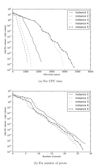
We implemented the simplex algorithm and tested it on five instances of the inventory management problem of Example 1. Recall that b, K, c, h, M denote the per-unit price, the fixed ordering cost, the per-unit ordering cost, the per-unit inventory cost, and the maximum ordering level, respec-tively, and let ddenote the expected demand in one period. The parameters of the five instances were (b, K, c, h, d, M) = (15,3,5,0.1,2,4), (10,5,7,0.1,2,4), (10,3,5,0.2,2,4), (10,3,5,0.2,2,5), (10,3,5,0.2,3,5), respectively. For all instances, demand in each period follows Poisson distribu-tion with the specified expected value. We used discount factor α = 0.9. The simplex algorithm was written in Python and ran on 2.93 GHz Intel Xeon CPU.
Figure 1 shows cost improvement of the simplex algorithm for the above instances of the inventory management problem as a function of (a) CPU time and (b) number of pivot operations. The vertical axis of Figure 1 is the difference between the objective function value of (D) of policies obtained by the simplex algorithm and the optimal objective function value. Fors∈ S, the initial basic action σ1(s) was the remainder ofs+ 3 divided by M. The objective function values of each policy were estimated by computingPN
s=1β(s)yN(s) for increasingN until the change of the value
in consecutive iterations was less than a threshold, where yN is obtained by solving (18).
Figure 1 illustrates that for all instances, the difference between the objective function value of poli-cies and the optimal value decreased monotonically and converged to zero. As shown in Figure 1b, the algorithm converges at similar rates for all instances as the number of iterations increases, but CPU time of one iteration is longer on average for instances 4 and 5 as shown in Figure 1a, possibly because of the higher maximum ordering level.
6
Discussion and Future Research
It is a natural next step to compare the simplex algorithm to the existing methods for countable-state MDPs. However, it is not straightforward how to make an empirical comparison. Aside from deciding how to implement those algorithms in a fair manner and which problem instances to try, another important issue is the cost of data acquisition. As those algorithms proceed, they require transition probabilities and rewards from more states. In practice, obtaining the problem data can be expensive. For example, if an algorithm converges to optimality in value faster than another algorithm but requires significantly more data, then it is not clear which one is a better solution method.
0 1000 2000 3000 4000 5000 6000 CPU time (secs)
10-9
10-8
10-7
10-6
10-5
10-4
10-3
10-2
10-1
100
101
102
(obj ftn value) - (opt value)
instance 1
instance 2
instance 3
instance 4
instance 5
(a) For CPU time
0 5 10 15 20 25 30
Number of pivots 10-9
10-8
10-7
10-6
10-5
10-4
10-3
10-2
10-1
100
101
102
(obj ftn value) - (opt value)
instance 1
instance 2
instance 3
instance 4
instance 5
[image:24.612.142.471.115.648.2](b) For number of pivots
would also be incomplete.
This paper generalized the LP approach in [8] to CILP formulations of a more general class of MDPs and introduced a simplex-type algorithm to a class of CILPs with less structure than those in the literature. To extend the LP approach of this paper to a more general class of CILPs, one would have to understand what aspects of the CILPs considered in this paper enabled the success of the LP approach. To be more precise, one needs to analyze what characteristics of the assumptions in Section 2.1 and the dynamic programming structure in the coefficient matrix (14) of (D) made it possible to establish the standard LP results and devise the simplex algorithm.
References
[1] C. Aliprantis and K. Border. Infinite-dimensional analysis: a hitchhiker’s guide. Springer-Verlag, Berlin, Germany, 1994.
[2] E. Altman. Constrained Markov decision processes. Chapman and Hall, CRC, 1998.
[3] E. J. Anderson and P. Nash. Linear programming in infinite-dimensional spaces: theory and applications. John Wiley and Sons, Chichester, UK, 1987.
[4] R. Cavazos-Cadena. Finite-state approximations for denumerable state discounted Markov decision processes. Applied Mathematics and Optimization, 14:1–26, 1986.
[5] E. Feinberg and A. Shwartz. Handbook of Markov decision processes. Kluwer International Series, 2002.
[6] A. Ghate. Duality in countably infinite linear programs. 2014. Working paper.
[7] A. Ghate, D. Sharma, and R. L. Smith. A shadow simplex method for infinite linear programs. Operations Research, 58:865–877, 2010.
[8] A. Ghate and R. L. Smith. A linear programming approach to nonstationary infinite-horizon Markov decision processes. Operations Research, 61:413–425, 2013.
[9] J. Harrison. Discrete dynamic programming with unbounded rewards. Annals of Mathematical Statistics, 43:636–644, 1972.
[10] O. Hern´andez-Lerma. Finite-state approximations for denumerable multidimensional state discounted Markov decision processes. Journal of Mathematical Analysis and Applications, 113:382–389, 1986.
[11] S. Lippman. On dynamic programming with unbounded rewards. Management Science, 21:1225–1233, 1975.
[12] M. L. Puterman. Markov decision processes: Discrete stochastic dynamic programming. John Wiley and Sons, New York, NY, USA, 1994.
[13] S. Resnick. A Probability Path. Birkh¨auser, 1999.
[14] H. E. Romeijn and R. L. Smith. Shadow prices in infinite dimensional linear programming. Mathematics of Operations Research, 23:239–256, 1998.
Mathematical Programming, 53:79–97, 1992.
[16] S. Ross. Introduction to stochastic dynamic programming. Academic Press, New York, NY, USA, 1983.
[17] H. Royden. Real Analysis. Macmillan Publishing Company, New York, 1988.
[18] W. Rudin. Principles of Mathematical Analysis. McGraw-Hill, Inc., 1976.
[19] T. C. Sharkey and H. E. Romeijn. A simplex algorithm for minimum cost network flow problems in infinite networks. Networks, 52:14–31, 2008.
[20] J. Wessels. Markov programming by successive approximations with respect to weighted supre-mum norms. Journal of Mathematical Analysis and Applications, 58:326–335, 1977.
[21] D. White. Finite state approximations for denumerable-state infinite horizon contracted Markov decision processes: The policy space method. Journal of Mathematical Analysis and Applications, 72:512–523, 1979.
[22] D. White. Finite state approximations for denumerable state infinite horizon discounted Markov decision processes. Journal of Mathematical Analysis and Applications, 74:292–295, 1980.
[23] D. White. Finite state approximations for denumerable state infinite horizon discounted markov decision processes: The method of successive approximations. In R. Hartley, L. Thomas, and D. White, editors,Recent Developments in Markov Decision Processes. Aca-demic Press, New York, 1980.
[24] D. White. Finite state approximations for denumerable state infinite horizon discounted Markov decision processes with unbounded rewards. Journal of Mathematical Analysis and Applications, 86:292–306, 1982.
[25] Y. Ye. The Simplex and policy-iteration methods are strongly polynomial for the Markov decision problem with a fixed discount rate.Mathematics of Operations Research, 36:593–603, 2011.
A
Derivation of (D) and Proof of Strong Duality
Here we provide some intuition behind problem (D) by illustrating its relationship to the MDP problem. We also prove strong duality between (P) and (D).
and rewards fors∈S˜and a∈ Aas:
˜
p(t|s, a),
αp(t|s, a) ifs6= 0, t6= 0 1−α ifs6= 0, t= 0
1 ifs=t= 0
,
˜
r(s, a),
(
r(s, a) ifs6= 0
0 ifs= 0.
Extend β by letting β(0) = 0 and π by arbitrarily choosing an action at state 0. The expected total reward is defined as:
˜
Vπ(β),E˜πβ
" ∞ X
n=0
˜
r( ˜Sn,A˜n)
#
,
where ˜Pπβ and ˜Eπβ are defined similarly for the new MDP, and the processes {S˜n} and {A˜n} are also defined accordingly. Then it is easy to show thatVπ(β) = ˜Vπ(β) for any policy π. We call this the absorbing MDP formulation of the original discounted MDP. It is said to be absorbing since it has a finite expected lifetime before entering 0 under any policy, i.e.,EπβT = 1/(1−α)<∞for any policy π, where T = min{n ≥0 : sn = 0}. Since the original discounted MDP and its absorbing MDP formulation can be considered equivalent, we use the same notation for both; it will be clear which one is discussed from the context.
For s∈ S and a∈ A, the occupancy measure of the state-action pair is denoted as Qβπ(s, a) and defined as the expectation of the number of visits to (s, a) until entering the absorbing state 0 under policy π with the initial state distributionβ, that is, for any s∈ S and a∈ A,
Qβπ(s, a),Eβπ
T−1 X
n=0
1{Sn=s, An=a}=Eπβ
∞
X
n=0
1{Sn=s, An=a}=
∞
X
n=0
Pπβ{Sn=s, An=a},
(29) where the last equality is due to Proposition 2.5. (An equivalent alternative interpretation of the occupancy measure is as the total expected discounted time spent in different state-action pairs in the original discounted MDP.)
It is well known (e.g., Theorem 8.1 of [2]) that for any policy π, there exists a stationary policyσ
such thatQβπ =Qβσ, namely,
σ(a|s) = Q β π(s, a)
P
b∈AQ
β π(s, b)
, (30)
whereσ(a|s) denotes the probability of σ choosing aats. This result implies that Q=QM =QS where Q,QM, andQS denote the sets of occupancy measures of all policies, Markov policies, and stationary policies, respectively.
It is also well known (e.g., Theorem 11.3 of [5] and Corollary 10.1 of [2]) that QS coincides with the set of nonnegative and summable solutions of the following set of equations:
A
X
a=1
x(s, a) =β(s) +α ∞
X
t=1
A
X
a=1
p(s|t, a)x(t, a) for s6= 0. (31)