Argo Data Mean Field Modeling

(1)

Argo Data Mean Field Modeling

by

Han Wu

A thesis submitted in partial fulfillment of the requirements for the degree of

Bachelor of Science (Honors Statistics) in The University of Michigan

2018

Advisors:

(2)

c

Han Wu 2018

(3)

(4)

ACKNOWLEDGEMENTS

Thanks to all the people who made this thesis possible, in particular Professor

Tailen Hsing and Professor Stilian Stoev for their help, guidance and insights, my

brother for working with me together and my family on the other side of the ocean

(5)

LIST OF FIGURES

Figure

2.1 Float Trajectory . . . 5

2.2 Cycle Variable Plots . . . 6

2.3 Cycle Time Series Plots . . . 6

3.1 B-spline basis functions . . . 11

3.2 One place for great variability . . . 15

4.1 Mixed layer depth and thermocline . . . 20

4.2 Mean field curve and derivative at (34.5N, 159.5E), January . . . . 21

4.3 Mean field curve and derivative at (34.5N, 159.5E), April . . . 22

4.4 Mean field curve and derivative at (34.5N, 159.5E), July . . . 22

4.5 Mean field curve and derivative at (34.5N, 159.5E), October . . . . 23

4.6 Mean field curve and derivative at (34.5N, 159.5E), December . . . 23

5.1 Mean field plot for 50db, January . . . 26

5.2 Mean field plot for 50db, February . . . 26

5.3 Mean field plot for 50db, March . . . 27

5.4 Mean field plot for 50db, April . . . 27

5.5 Mean field plot for 50db, May . . . 28

5.6 Mean field plot for 50db, June . . . 28

5.7 Mean field plot for 50db, July . . . 29

5.8 Mean field plot for 50db, August . . . 29

5.9 Mean field plot for 50db, September . . . 30

5.10 Mean field plot for 50db, October . . . 30

5.11 Mean field plot for 50db, November . . . 31

(8)

ABSTRACT

Argo Data Mean Field Modeling

by

Han Wu

Professor Tailen Hsing, Professor Stilian Stoev

In this thesis, we provide a new method for modeling the mean field of the Argo

data set. We use a non-parametric method which could take vertical dependence into

account and has a clear closed form solution. Existing mean fields suffer from the

drawback that they are not continuous and focus on specific pressure levels. We also

use the mean field to investigate the thermocline and mixed layer depth, which are

of great interests among oceanographers. They can be easily analyzed by existing

method if we have a closed form expression of the temperature-pressure curve. We

also illustrate how we did the computations and give some plots about the mean field.

(9)

CHAPTER I

Introduction

1.1

Introduction

Argo data set is collaboratively collected by many countries. It measures salinity,

temperature and pressure of the ocean by floats, which are deployed at certain location

and then start to drift randomly. The floats collect data in every 10 days. In each

cycle, the time information is also recorded when the float comes to the surface.

It collects data as deep as 2000 meters whereas traditional data sets only focus on

surface areas. Also, the resolution of the floats is getting finer. The current resolution

is 3◦×3◦ so on average there is one float in every 3◦×3◦ grid. There are still some

implementation issues scientists are trying to improve upon. For example, there are

fewer floats in the polar area and in the south hemisphere in general, partly because

there are fewer countries in these areas. Also, the current scheme of Argo measures

the time when the float comes to the surface so the temporal information is not

accurate for data collected in the deep ocean. The data set is of great interests to

(10)

1.2

Roemmich-Gilson Argo Climatology

In this section, we give an introduction to the Roemmich-Gilson (RG) mean field,

which is considered the gold standard for researchers interested in Argo. More details

about the RG project could be found in [Kuusela and Stein (2017)].

The website of the product http://sio-argo.ucsd.edu/RG_Climatology.html

provides a summary, “A basic description of the modern upper ocean based entirely on

Argo data is available here, to provide a baseline for comparison with past datasets

and with ongoing Argo data, to test the adequacy of Argo sampling of large-scale

variability, and to examine the consistency of the Argo dataset with related ocean

observations from other programs.” [Roemmich and Gilson (2017)].

According to their website of the product, “The RG Argo Climatology uses

weighted least-squares fit to the nearest 100 Argo profiles within a given month to

estimate the mean field.” They fit the model on some fixed pressure levels for each

lattitude-longitude grid point. The regression function includes first and second terms

of the latitude, longitude and pressure as well as fourier basis to account for the

sea-sonal cycle. Specifically, the regression function given in Kuusela and Stein (2017) is

as follows

m(xlat, xlon, z, t) =β0+ [first and second order terms of xlat,xlon and z]

+ 6 X

k=1 γksin

2πk t 365.25

+δkcos

2πk t 365.25

wherexlatis latitude,xlonis longitude,zis pressure andtis time in days within a year.

This function is fitted to the nearest 3× 12×100 neighbors, where 3 refers to the 3

nearby pressure levels and 12 refers to the calendar months. The nearest neighbors

are identified across the whole data set and are assigned with weights depending on

their distances with the grid point. “Once fitted, the regression function is evaluated

(11)

(12)

CHAPTER II

Float Analysis

This chapter describes a naive way of analyzing individual floats using time series.

However, as we will see this analysis can only serve as a way to explore the data.

The model cannot be generalized, and the analysis is not definitive. So, after this

preliminary attempt we will focus on modeling the mean field of temperature.

2.1

Float Analysis

We focus on one specific float. We try to model one typical cycle of the float.

Note that the website

http://www.argodatamgt.org/Access-to-data/Description-of-all-floats2 has descriptions of all the floats, both active and inactive. So we could

have a look to see what a typical cycle looks like. The basic idea of the analysis is to

estimate a time series model using one or several cycles and then use the estimated

model to predict the remaining cycles. The model we use is vector auto-regressive

(VAR) model. One thing to note is that this model is not perfectly suitable as the

movement of floats is non-stationary. We also tried VARMA model but it turned out

that this model improves nothing but complexity. The trajectory of one such float is

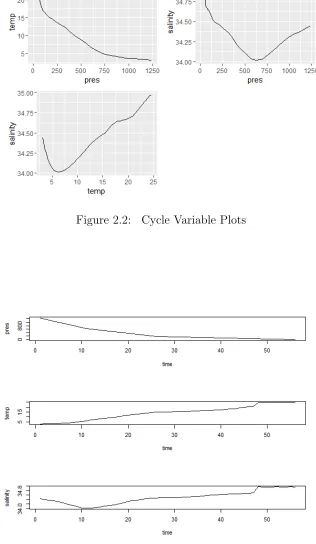
shown in figure 2.1. The typical cycle variable plots is figure 2.2. The typical time

series plot of each cycle is figure 2.3.

(13)

[image:13.612.169.481.72.230.2]

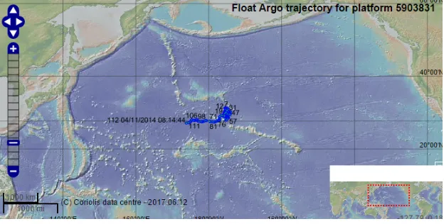
Figure 2.1: Float Trajectory

Figure courtesy of Argo data management site,

http://www.argodatamgt.org/Access-to-data/Description-of-all-floats2

the first p observations (corresponding to the deepestp pressure levels) in each cycle

since the model requires pprevious observations to make a prediction. The details of

the procedure are given below.

2.2

Different ways of handling cycles

2.2.1 Using one cycle

In this setting, we use the data from only one cycle to estimate the model. We first

perform an order selection. We should choose the last small p-value in the sequential

p-value list provided by the MST package. We also want AIC, BIC and HQ values

to be small. Order 3 is sufficient in most of the time. We fit the model and predict

the subsequent cycles. After getting models from each cycle, we compare the model

parameters and they are pretty different. However, the errors are quite similar.

2.2.2 Using half data

In this setting, we naively combine half of the data without any modification and

it turns out this approach has larger error rates than previous one, which suggests

(14)

[image:14.612.171.483.104.329.2] [image:14.612.163.479.123.667.2]

Figure 2.2: Cycle Variable Plots

(15)

of the VAR model tells us that it uses least squares so the problem comes from the

first three observations of each cycle. Based on this observation, we tried a new way

of combining the data.

2.2.3 New way of combining the data

In this setting we do not omit the first three observations and use the function

in the package MTS. Instead, we perform the least square and treat every possible

group of four data points as an observation coming from the model. Using the first

half as training data, the performance is better than the method in last section.

2.2.4 Miscellaneous

We also looked at errors of the last five observations in each cycle. The predictions

are worse especially for pressure. This is expected since near the surface the changes

are more abrupt than in deep water. This phenomenon also suggests that we should

take a look at the plots of the cycles to visualize them and shift our attention to

smaller pressure area.

2.3

Summary

In summary we found that VAR model works very well for modeling salinity no

matter how many cycles we use as training data. The average prediction error of

temperature is around 10% for the float we chose. However, VAR model is not a

natural way to model all floats as there is no VAR model that works uniformly well.

There is no reason to assume that a float drifting near equator obeys the same model

as a float drifting near the pole. Also, for some floats that drifts for a very long

distance the analysis becomes problematic. However, one thing we get from this

(16)

terms of pressure, which means vertical dependence is crucial. This motivates us to

(17)

CHAPTER III

Mean Field Modeling

3.1

Introduction

In this chapter, we introduce a functional data approach to model the mean

tem-perature field across the entire ocean. Other existing methods for computing the

mean field involve a fixed given pressure level. We propose a nonparametric approach

using B-splines, which smoothly incorporates all pressure levels. The approach has

many advantages including: it has a closed form solution, it is relatively easy to

compute and it allows us to visualize the results.

3.2

B-Splines

We first give a short introduction to B-splines. B-splines are particularly useful

basis functions for the space of smooth piecewise polynomial functions referred to as

splines. Any spline function of given degree can be expressed as a linear combination

of B-splines of that degree. Also, we have closed form expression of the basis we

will use. The B-splines are defined as follows [Wasserman (2006)]. Let ξ0 = a and

ξk+1 =b. Define new knotsτ1, . . ., τM such that

(18)

and

ξk+1≤τk+1+M ≤ · · · ≤τk+2M (3.2)

The choices for knots beyond the boundary are arbitrary and could be chosen to equal

toa and b respectively.

B-spline basis functions are defined recursively, we first define

Bi,1(x) =       

1, if τi ≤x < τi+1

0, otherwise

for i= 1, ..., k+ 2M −1.

Form ≥2 and m≤M, we define

Bi,m(x) =

x−τi

τi+m−1−τi

Bi,m−1(x) +

τi+m−x

τi+m−τi+1

Bi+1,m−1(x)

If the denominator is 0 then we define the function to be 0.

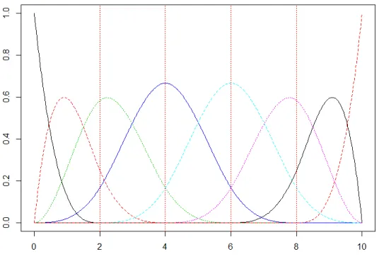
The following figure 3.1 shows examples of B-spline basis functions with order 4 and

knots at 0, 2, 4, 6, 8, 10.

Theorem

The functions {Bi,4(x), i= 1, ..., k+ 4} are a basis for the set of cubic splines. They

are called the B-spline basis functions.

A proof of this theorem can be found in Carl de Boor’s notes [de Boor (2017)].

Now suppose ˆf is the spline estimator. We have

ˆ f(p) =

N

X

j=1

βjBj(p)

where B1, . . .,BN are basis functions, we need to find β = (β1, . . . , βN). So we need

to minimize

(19)

[image:19.612.191.459.98.281.2]

Figure 3.1: B-spline basis functions

where B = (Bj(pi)) and Ωjk =

R

B_j00B_k00. Taking the derivative we have

ˆ

β = (BTB +λΩ)−1BTY

The above formula is used in the fda package. One thing to note is that using B-spline

basis functions could help us speed up the computation ofβ compared to using other

basis. This is because by induction we could show that Bi,4 = 0 for x /∈ [τi, τi+M],

so the support of B-spline basis functions is at most 5 knots [Hastie et al. (2009)].

Thus, theB matrix in the above formula is lower 4-banded. Consequently the matrix

(BT_B ₊_λ_{Ω) is 4-banded and hence its Cholesky decomposition can be computed}

(20)

3.3

Models

3.3.1 The data

The data we use comes from [Kuusela (2018)], it contains roughly one million

profiles from year 2007 to year 2016. There is a strict requirement for selecting the

data, namely all cycles with big gaps in pressure readings are discarded. Whether

this is sensible is yet to be determined with further evaluation. The profiles consist

of separate lists for Julian date, latitude, longitude, pressure and temperature. Note

that here we already ignored salinity. Each element in the first three lists is a single

scalar since as we said earlier, the location and time information are only assessed

once the float comes to the surface. Each element in the latter two lists is a vector

and its length varies according to the technical aspect of the float. Specifically, theith

profile consists of (JULDi,LATi,LONi,(Pi,j)jn=1i ,(Ti,j)nj=1i ). The data are in Matlab.

We used the R.matlab package in R to transform Matlab data structures to R.

3.3.2 Introduction and motivation

Besides what we present in the last chapter, the idea of modeling the mean comes

from two considerations. The first one is the intuition that in general the pattern of

temperature should roughly be the same across different years. The second one is the

fact that the data set is rather sparse, so modeling the mean is crucial for further

data analysis.

A natural idea is using regression for each pressure level which is what is done

by Roemmich and Gilson, but as explained in the introduction, it is hard to produce

a continuous mean field as a function of pressure. Also, the computation will be

challenging and the model is complicated which compromises interpretability. We

use the idea that we could borrow strength from nearby profiles to get information

(21)

interested in. We use nearby cycles in a way to produce the mean for a point where

all the cycles considered will lie in a circle with some radius centered at this point.

Depending on the degree of similarity with the point we consider, we should give

them different weights. Thus, the idea is to use two weights, one for time and one for

location. The overall weight is the product of the two.

We use a non-parametric approach here to model the pressure temperature curve

and take advantage in later sections of the closed form we have. One thing to note is

that this approach can be extended to predict at a location and time not covered by

any float. Thus, our methodology addresses the important issue of sparsity.

3.3.3 Model specification

In this section we elaborate on the smoothing methodology we developed.

Suppose we are given a point (time, s) wheretime∈[0,365.25) denotes the time

in the year, which is calculated as follows.

time= JULD−

JULD 365.25

×365.25

where JULD is the Julian Date in original data set. s is the location consisting of

latitude and longitude, i.e. s = (lat, lon). We will model the mean locally, i.e. all

the data from each year in a window have similar means. We produce the baseline

model locally using linear combinations of B-spline basis functions. So the model is

as follows:

T =f(p) +

where f is a linear combination of B-spline basis functions as well as a linear term

and intercept term, is the noise with mean zero (modeling this would be further

(22)

supported in the interval [0, p0] with order m. We have

f(p) =β1ψ1(p) +· · ·+βm+2ψm+2(p)

We want to minimize the residual sum of squares but for each profile we want to use

the average of residual sum of squares so that the result is not dominated by profiles

with much more pressure levels than others.

Now, given a window size ‘hspace’ for location and ‘htime’ for time, we consider

the profiles whose locations lie inside the circle centered at the given location point

(lat, lon) with radius ‘hspace’ and whose times are in the interval [time-htime, time

+ htime]. Specifically, suppose i = 1, . . . , N denote the index of profiles in a given

window and j = 1, . . . , ni denote the pressure levels of this profile (ni is the number

of data points in this profile), then for profile i we have the residual sum of squares

1 ni

ni

X

j=1

Ti,j− m+2 X

k=1

βkψk(pi,j)

!2

Now as mentioned above, the weight function is the product of weight of time and

weight of location. For time kernel we employed two in our later computation,

Epanechnikov kernel and box kernel. For the Epanechnikov kernel, we have

wt(time, t) =

       3 4(1−(

|t−time| htime )

2₎_, _if |t−time|

htime ≤1

0, otherwise,

For the box kernel we simply put weight 1 for all time points in the interval i.e.

wt(time, t) =

      

1, if |t−time|_htime ≤1

(23)

For the weight of space, we only use Epanechnikov kernel parametrized by ‘hspace’,

i.e. for two locations s1 = (lat1, lon1) ands2 = (lat2, lon2), we have

ws(s1, s2) =        3 4(1−(

(lat2−lat1)2+(lon1−lon2)2

hspace2 )), if

(lat2−lat1)2+(lon1−lon2)2

hspace2 ≤1

0, otherwise,

The reason for this is that from our empirical analysis, space variability is huge for

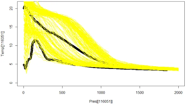
some places and time variability has less influence on the result. For illustration, see

[image:23.612.163.476.309.485.2]

figure 3.2. The lower thick black line is the true curve, and the upper black one is the

Figure 3.2: One place for great variability

Upper balck line is the mean curve and the lower black line is the curve plotted using raw data. Yellow lines are cycles used to produce the mean curve

mean we produced. We see huge variability here. So it is better to model the mean

in a smaller region and not using uniform kernel.

We will weight the average of the residual sum of squares from different profiles

by its weight. We want to find the best parameter β, so

ˆ

β = argmin

β∈Rm N X i=1 1 ni ni X j=1

Ti,j − m

X

k=1

βkψk(pi,j)

!2

(24)

where

wi =wt(time, ti)ws((lati, loni), s)

and β depends on the location s= (lat, lon), time, hspace and htime.

The value for hspace is subject to our own choice. We tried 5 for producing the

mean field and also 3 to see how well our mean field prediction will be compared to

Roemmich-Gilson mean field. The reason to choose radius of 5 is because we want to

include more data and empirically this is a pretty decent choice. The reason for using

the radius 3 is twofold. First, Argo is roughly distributed at a resolution of 3 by 3

grid. Second, because of the huge variability it is better to choose a smaller radius

if we want a better mean field in pure prediction point of view. We use a month as

time window because Rommeich Gilson mean field focuses on monthly mean. One

thing to note is that these are just hyper-parameters so we could change them and

rerun our code to get a different mean field. If we write

β = [β1,· · ·, βm]T,Ψi =

     

ψ1(Pi,1) · · · ψm(Pi,1) ..

. . .. ...

ψ1(Pi,ni) · · · ψm(Pi,ni)

     

, Ti = [Ti,1,· · · , Ti,ni]

T _(3.4)

Then we can write the above minimization problem in a compact form

ˆ

β(lat,lon,time; hspace,htime) = argmin

β∈Rm

N

X

i=1

kTi−Ψiβk2

wi

ni

(3.5)

Taking the gradient of right hand side of (3.5) we have

∂ ∂β

N

X

i=1

kTi−Ψiβk2

wi

ni

= ∂

∂β(Ti−Ψiβ)

T₍_T

i−Ψiβ)

wi ni = N X i=1

(−2ΨT_i Ti+ 2ΨTi Ψiβ)

wi

(25)

Setting the above expression to zero we have N X i=1 wi ni

ΨT_i Ψ ! β= N X i=1 wi ni

ΨT_i Ti

so ˆ β = N X i=1 wi ni

ΨT_i Ψi

!−1 _N X

i=1 ΨT_i Ti

wi

ni

!

(3.6)

To predict the temperature we simply use

ˆ

Ti = Ψiβˆ (3.7)

Remark

We have investigated some variations of the model.

• We tried to add the seasonal cycles into the model as Rommiech and Gilson did.

Recall that RG method involves such terms for each fixed pressure level. Since

we are considering different pressure levels together, given the large number of

parameters it is hard to incorporate the seasonal consideration in the model.

Also, given the performance of our mean field, we think it is unnecessary to

increase the complexity of the mean field model.

• We also tried to incorporate time of the day into the model, i.e. giving more

weight to profiles that have similar time of the day with the target profile.

This is feasible. We used the triweight kernel and also considered the influence

of pressure. When the pressure is low there should be stronger influence on

temperature coming from time of the day. Although this does improve the fit

a little bit for the first few observations having small pressures, it has virtually

(26)

3.4

Producing the mean field

One advantage for using the B-spline basis function approach is that we have a

closed form solution of ˆβ. However, to calculate ˆβ we need to sum over i, which

involves a loop and its implementation in R is prohibitively slow. We overcome this

bottleneck by using the package Rcpp, which allows us to implement the loop in C++

and integrate the function in R. We also take advantage of the fda package in R that

is very convenient for B-splines. We use the fda package mainly for producing the Ψ

(27)

CHAPTER IV

Thermocline and Mixed Layer Depth

4.1

Introduction

In this chapter, we introduce the concept of thermocline and mixed layer depth.

These are very important concepts in oceanology research. Having computed the

mean field, we can use it to do some basic explorations of the thermocline and mixed

layer depth at various locations and times of the year.

4.2

Basic Concepts

Informally, Figure 4.1 depicts the concepts of mixed layer depth and thermocline.

We give the definitions of these terms presented in the website of University of Illinois

WW2010 Project, http://ww2010.atmos.uiuc.edu/(Gh)/wwhlpr/thermocline.rxml.

“The thermocline is the transition layer between the mixed layer at the surface

and the deep water layer. The definitions of these layers are based on temperature.

The mixed layer is near the surface where the temperature is roughly that of

surface water. In the thermocline, the temperature decreases rapidly from the mixed

layer temperature to the much colder deep water temperature.

The mixed layer and the deep water layer are relatively uniform in temperature,

(28)

[image:28.612.261.387.88.272.2]

Figure 4.1: Mixed layer depth and thermocline

Image from the University of Illinois WW2010 Project, http://ww2010.atmos.uiuc.edu/(Gh)/wwhlpr/thermocline.rxml

4.3

Identifying Thermocline

There are several ways to identity the thermocline region. Basically, we need

to find both the upper bound (aka mixed layer depth) of the thermocline and the

lower bound of the thermocline. Holte and Talley [Holte and Talley (2009)] give a

comprehensive review of the existing methods to determine mixed layer depth and

posit a new algorithm. We find those methods tedious and difficult to implement.

Rather, we find the approach inJiang et al. (2017) more interesting. The basic idea

is as follows.

They first define the concept of the thermocline strength, which refers to the

quotient of temperature difference divided by depth difference. They use 0.2C/m

as the threshold value to judge thermocline. If the maximum regional strength is

smaller than 0.2C/m, they will claim that there is no thermocline in this region

Jiang et al. (2017). In our case, we focus on 1-m interval, i.e. pressure level vector

(0,1,2,· · · ,2000). For each pressure level, we have the derivative calculated from the

(29)

than or equal to 0.2, we tag it as thermocline. Following this method, we can have

several preliminary thermocline regions. We first throw away all the regions with

thickness less than 5m. Then we merge all the thermoclines with distance less than

5m.

This method is easy to implement and avoids some hard to understand technical

details.

4.4

Plots of derivatives and mean field curves

In this section, we provide some plots of both derivatives and original mean field

[image:29.612.115.560.349.530.2]

curves.

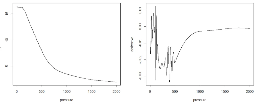
Figure 4.2: Mean field curve and derivative at (34.5N, 159.5E), January

Observations

1. It is hard to capture the fluctuations or stability sometimes near the surface,

which will make determining the upper bound of the thermocline (also called Mixed

Layer Depth or MLD) harder.

2. When our mean field estimate looks very different from the real curve, most of

(30)

[image:30.612.113.561.97.276.2]

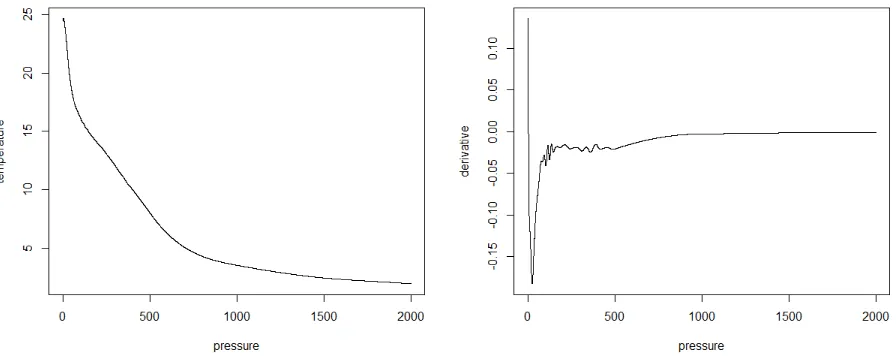
Figure 4.3: Mean field curve and derivative at (34.5N, 159.5E), April

Figure 4.4: Mean field curve and derivative at (34.5N, 159.5E), July

4.5

Common methods in oceanology to determine MLD

From the introduction part of Holte and Talley (2009), the most widely favored

and simplest scheme for finding the MLD is the threshold method. “Threshold

meth-ods search for the depth at which the temperature or density profiles change by a

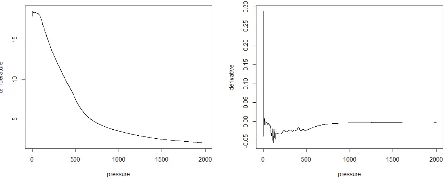
[image:30.612.113.561.346.524.2]

(31)

[image:31.612.110.561.98.275.2]

Figure 4.5: Mean field curve and derivative at (34.5N, 159.5E), October

Figure 4.6: Mean field curve and derivative at (34.5N, 159.5E), December

threshold value is still an open problem. Some scientists discovered that larger

thresh-old values might overestimate the MLD of individual profiles and similarly smaller

value of 0.1 degree celsius underestimates the MLD. In de Boyer Montgut et al. 0.2

was suggested as the optimal value (reference level at 10m to avoid diurnal heating).

Gradient methods work like threshold methods. They assume that there is an abrupt

[image:31.612.112.561.344.525.2]

(32)

values. Commonly used value is 0.025 C/m. Note that, density could also be used

for both methods.

Threshold and gradient methods have limitations because their performances

de-pend largely on the reference and threshold values. Also, it is difficult to find a value

that is uniformly well for all the profiles in the ocean. In general, some scientists have

argued that density criterion is more reliable for finding MLD than a temperature

criterion [Holte and Talley (2009)].

4.6

The merit of our approach

One thing to note is that most of the literature and research on MLD and

thermo-cline have to rely on raw data. They will apply existing methods to the raw data and

estimate the MLD and thermocline region. This is a significant limitation because

it confines the methods to the data collecting technology. However, if we use the

functional data approach to get a closed form solution of the mean as a function of

pressure, we could do our analysis at locations where data are not even collected. By

(33)

CHAPTER V

Mean Plots of Gridded Files

5.1

Introduction

Based on the method we described in Chapter 3, we produced a grided mean field.

We used the grid offered by Roemmich and Gilson. Namely, we divided the whole

world into 1◦ ×1◦ grid and compute a mean temperature curve for each grid as a

function of pressure and time. We set the time window to 30 days and space window

to 5 degrees with box kernel on time and Epanechnikov kernel on space. The mean

field we calculated is for all the Argo data up to 2016. For each month and for each

spatial grid, we have a vector of coefficients in the B-spline basis as well as a mean

vector. Therefore, the final product we got is a multi-dimensional array.

5.2

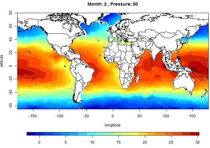
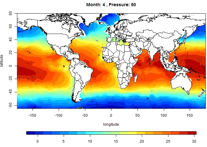
Mean Field Plots

In this section, we show some mean field plots for pressure level 50 db. Each plot

represents a mean temperature field of the ocean in a given month. The plots are

(34)

[image:34.612.151.485.116.345.2]

Figure 5.1: Mean field plot for 50db, January

[image:34.612.151.486.436.673.2]

(35)

[image:35.612.151.485.116.345.2]

Figure 5.3: Mean field plot for 50db, March

[image:35.612.151.486.435.673.2]

(36)

[image:36.612.151.485.116.344.2]

Figure 5.5: Mean field plot for 50db, May

[image:36.612.151.486.434.673.2]

(37)

[image:37.612.151.485.116.346.2]

Figure 5.7: Mean field plot for 50db, July

[image:37.612.151.485.434.673.2]

(38)

[image:38.612.151.485.116.343.2]

Figure 5.9: Mean field plot for 50db, September

[image:38.612.150.486.441.675.2]

(39)

[image:39.612.151.485.117.343.2]

Figure 5.11: Mean field plot for 50db, November

[image:39.612.151.486.438.674.2]

(40)

CHAPTER VI

Conclusion and Further work

We have demonstrated the convenience of having a closed form expression of our

estimated mean field and its power in other areas of analysis of Argo data. The mean

field is pretty flexible and careful choice of parameters could certainly improve the

prediction accuracy even if we only use mean field to predict the temperature. There

are some further works that can be done in the future. For example, how we could pick

location dependent bandwidths for the kernels and carefully cross validate the choice

of knots, order of basis functions on such a large scale. In terms of prediction, how

we could carefully model the residuals. We have looked at some empirical covariances

but have not proceeded with further analysis. The choice of covariance function is

crucial for successfully modeling the residuals. One challenge is the high-dimensional

feature of the data. For each window if we regard data points from each year as an

iid realization from the same process then the dimension is too large to use existing

method to estimate the model parameters. Further work on residual modeling would

(41)

(42)

BIBLIOGRAPHY

de Boor, C. (2017), B(asic)-spline basics, ftp://ftp.cs.wisc.edu/Approx/ bsplbasic.pdf.

de Boyer Montgut, C., G. Madec, A. S. Fischer, A. Lazar, and D. Iudicone (), Mixed layer depth over the global ocean: An examination of profile data and a pro-filebased climatology, Journal of Geophysical Research: Oceans, 109(C12), doi: 10.1029/2004JC002378.

Hastie, T., R. Tibshirani, and J. Friedman (2009),The Elements of Statistical Learn-ing: data mining, inference and prediction, 2 ed., Springer.

Holte, J., and L. Talley (2009), A new algorithm for finding mixed layer depths with applications to argo data and subantarctic mode water formation,Journal of Atmospheric and Oceanic Technology, 26(9), 1920–1939.

Jiang, Y., Y. Gou, T. Zhang, K. Wang, and C. Hu (2017), A Machine Learning Approach to Argo Data Analysis in a Thermocline, Sensors (Basel, Switzerland), 17(10), 2225.

Kuusela, M. (2018), https://github.com/mkuusela/PreprocessedArgoData.

Kuusela, M., and M. L. Stein (2017), Locally stationary spatio-temporal interpolation of Argo profiling float data,ArXiv e-prints.

Roemmich, and Gilson (2017), Roemmich-Gilson Argo Climatology, http:// sio-argo.ucsd.edu/RG_Climatology.html.

http://sio-argo.ucsd.edu/RG_Climatology.html

ftp://ftp.cs.wisc.edu/Approx/bsplbasic.pdf

https://github.com/mkuusela/PreprocessedArgoData.