Evolutionary techniques for updating query cost models
in a dynamic multidatabase environment
Amira Rahal1, Qiang Zhu1, Per- ˚Ake Larson2
1 Department of Computer and Information Science, The University of Michigan – Dearborn, Dearborn, MI 48128, USA
(e-mail:{arabi,qzhu}@umich.edu)
2 Microsoft Research, One Microsoft Way, Redmond, WA 98052, USA
(e-mail: [email protected])
Edited by L. Liu. Received: November 25, 2002 / Accepted: May 20, 2003 Published online: September 30, 2003 – cSpringer-Verlag 2003
Abstract. Deriving local cost models for query optimization
in a dynamic multidatabase system (MDBS) is a challeng-ing issue. In this paper, we study how to evolve a query cost model to capture a slowly-changing dynamic MDBS environ-ment so that the cost model is kept up-to-date all the time. Two novel evolutionary techniques, i.e., the shifting method and the block-moving method, are proposed. The former up-dates a cost model by taking up-to-date information from a new sample query into consideration at each step, while the latter considers a block (batch) of new sample queries at each step. The relevant issues, including derivation of recurrence updat-ing formulas, development of efficient algorithms, analysis and comparison of complexities, and design of an integrated scheme to apply the two methods adaptively, are studied. Our theoretical and experimental results demonstrate that the pro-posed techniques are quite promising in maintaining accurate cost models efficiently for a slowly changing dynamic MDBS environment. Besides the application to MDBSs, the proposed techniques can also be applied to the automatic maintenance of cost models in self-managing database systems.
Keywords: Multidatabase – Query optimization – Cost
model – Evolutionary technique – Self-managing database
1 Introduction
A multidatabase system (MDBS) integrates data from multi-ple component (local) databases. A major challenge, among others [6,8,10,11,16], for performing global query optimiza-tion in an MDBS is that some local informaoptimiza-tion required by global query optimization, such as local cost models, may not be available at the global level. However, the global query optimizer needs such local cost information to decide how to decompose a global query into local queries and where to execute the local queries.
Research supported by the US National Science Foundation under Grant # IIS-9811980 and The University of Michigan under OVPR and UMD grants.
Several techniques to derive cost models for an auto-nomous local database system (DBS) at the global level in an MDBS have been proposed in the literature recently. Du et al. proposed a calibration method that makes use of the observed costs of some special queries run against a special synthetic calibrating database to deduce necessary local cost parameters [5]. Gardarin et al. extended Du et al.’s method so as to calibrate cost models for object-oriented local DBSs in an MDBS [7]. Zhu and Larson proposed a query sampling method that develops regression cost models for local query classes based on observed costs of sample queries run against actual user databases [21,24,25]. Zhu and Larson also intro-duced a fuzzy method to derive fuzzy cost models in an MDBS based on fuzzy set theory [23]. Naacke et al. suggested an ap-proach to combining a generic cost model with specific cost information exported by wrappers for local DBSs [12]. Adali et al. suggested maintaining a cost vector database to record cost information for every query issued to a local DBS [1]. Roth et al. introduced a framework for costing in theirGarlic
federated system [15].
0 500 1000 1500 2000 2500 3000 3500 4000 4500 5000 10
20 30 40 50 60 70
Buffer Size (in Blocks)
Query Cost (Elapsed Time in Sec.)
Environment: SunOS 5.1 on SUN UltraSparc 2 with 128 MB memory Tables: R1(a1, a2, ..., a9) −− 50,000 tuples
R2(a1, a2, ..., a11) −− 100,000 tuples Query: SELECT /*+first_rows/ R2.a1, R2.a6
FROM R1, R2
WHERE R1.a7 = R2.a7 AND R1.a9 = 164 AND R2.a2 > 148
Query cost change: 77.6%
Fig. 1.Query cost affected by buffer size in Oracle 8.0
environmental factors for the network in an MDBS that were considered in [18].
Clearly, the steady factors (Type III) usually do not cause any problem for a query cost model since they rarely change. To take the frequently changing factors (Type I) into consid-eration for estimating query costs, Zhu et al. suggested three techniques in [19,20], i.e., the qualitative approach, the frac-tional analysis approach, and the probabilistic approach. The qualitative approach is suitable for estimating the cost of a small query using a cost model with a qualitative variable indicating system contention states. The fractional analysis approach is suitable for estimating the cost of a large query by analyzing cost fractions in a dynamic environment following a prior known load curve. The probabilistic approach is suitable for estimating the cost of a large query based on Markov chain theory in a randomly changing dynamic environment.
However, no research has been done on estimating local cost parameters in a slowly changing dynamic environment (caused by factors of Type II). Although such an environ-ment may not change dramatically during the execution of one query, the costs of the same query executed at different times in the environment can be significantly different. Fig-ure 1 shows that the cost of a query in Oracle 8.0 can change dramatically as the buffer size (a configuration parameter) is adjusted by a database administrator over time. Note that the performance change could be even more dramatic if the query were performed against a larger database on a faster machine with larger memory. Compared to the factors of Type I, the factors of Type II change gradually rather than rapidly. But a significant change may be observed after a certain period of time. An obsolete cost model may cause a query optimizer to choose an inefficient execution plan for a query, which would lead to a serious performance problem. The question now is how to obtain accurate query cost estimates at all times in such a slowly changing environment.
In this paper, we tackle this challenge by evolving a cost model to capture the slowly changing environment so that the cost model is kept up-to-date all the time. One direct method of keeping a cost model updated is to periodically rebuild the cost model by the query sampling method [21]. However, the
overhead of such a rebuilding approach is high. To reduce the overhead, we propose two new evolutionary techniques, i.e., a shifting method and a block-moving method. The key idea is to develop recurrence updating formulas to adjust a cost model at each updating step rather than rebuild the cost model from scratch every time so that some common work done previously can be reused. The shifting method evolves a cost model more smoothly but takes more overhead as compared with the block-moving method. Evolving a cost model to capture a dynamic database environment is our novel approach; it has not been found in literature.
The rest of the paper is organized as follows. Section 2 discusses the idea of cost model evolution and the direct re-building approach. Section 3 introduces the shifting method. Section 4 presents the block-moving method. Section 5 con-siders some implementation issues. Section 6 shows some ex-perimental results. Section 7 summarizes the conclusions.
2 The rebuilding approach
In the query sampling method [21,25], queries that can be per-formed on a local DBS are first grouped into homogeneous query classes, and a cost model is then developed for each query class based on the observed costs of sample queries drawn from the class via multiple regression analysis in statis-tics. Such a cost model captures the performance behavior of queries from the relevant class for a specific environment in which the sample queries were executed. If the environment has changed dramatically since the cost model was developed, the cost model may become out of date. The question is how to keep the cost model up-to-date so that it always reflects the current environment.
Suppose we want to keep the cost modelM for a query class G up-to-date in a dynamic multidatabase environ-ment. Let the set of significant explanatory variables deter-mined by the query sampling method for the cost model be {x1, x2, . . . , xn}, e.g., the operand table size, the result table
size,1 the operand table tuple length, etc. Cost model M is then of the following form [24]:
y=β0+β1x1+β2x2+. . .+βnxn (1)
whereβi’s (0 ≤ i ≤ n) are the regression coefficients
de-termined by sample queries. Using the relevant value of each explanatory variablexj(1≤j≤n) for queryQinG, we can
estimate costyofQfrom Eq. 1. Note that the aim of this paper is not to develop a new cost modeling technique. Instead, it assumes that a cost model and its parameters are determined by the techniques presented in [24]. This paper focuses on de-veloping new techniques to efficiently adjust the coefficients in the cost model so that the environmental changes can be effectively captured.
In the rest of this paper, we adopt the following notation. A column vector is denoted byz using a lowercase letter. A row vector is denoted by the transposition of its corresponding column vectorzT. A matrix is denoted by a bold-faced capital letter (e.g.,A), and the inverse ofAis denoted byA−1. A
1
sample queries
sample data points
M M
M M
M (0)
(1) (2)
(3) (4)
...
...
...
...
...
...
...
modelscost
Q Q Q Q Q Q Q Q Q Q Q
t t t t t t t t t t t
d d d d d d d d d d d ~t
~t ~t
~t ~t
0 1 2 3 4 k−1 k k+1 k+2 k+3 k+4
0 1 2 3 4 k−1 k k+1 k+2 k+3 k+4 k
k−1
k+1 k+2
k+3
t0 t1
t2 t3
t4
time
...
periods
0 1 2 3 4 k−1 k k+1 k+2 k+3 k+4
[image:3.595.49.362.54.210.2]time
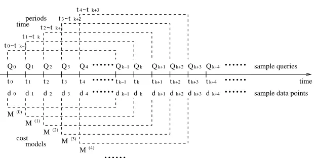
Fig. 2.Rebuilding up-to-date cost models
scalar value or variable is denoted by a normal lowercase letter (e.g.,b).
LetQi(i= 0,1,2, . . .) be a sample query fromGexecuted
at timeti. Letyibe the observed cost (elapsed time) ofQiand
xij be the observed value ofj-th variablexj (1 ≤ j ≤ n)
forQi. Let row vectorxTi = (1, xi1, xi2, . . . , xin). Note that
the first component “1” in vectorxT
i, which corresponds to
the constant term in Eq. 1, is used to simplify the cost for-mula derivation later on. We call pair(yi, xTi) as the
sam-ple data point (for samsam-ple query Qi) observed at time ti.
Hence we have a sequence of sample data points(y0, xT 0),
(y1, xT1), . . . (corresponding to the sequence of sample queries
Q0,Q1, . . . ) att0,t1, . . . .
Assume the sample size for multiple regression analysis in the query sampling method isk.2At timetk−1, we have
ksample data points (y0, xT
0),(y1, xT
1), . . . , (yk−1,xTk−1).
Applying the multiple regression analysis on these sample data points, we can obtain a cost modelM(0)that reflects the system performance behavior for query classGduring the time period
t0∼tk−1.
As mentioned before, the system environment may change significantly over time, although for our problem we assume that it changes slowly. If we keep usingM(0)to estimate the costs of queries executed at timetk,tk+1,tk+2, . . . , the es-timates may become progressively worse. To get better esti-mates, we need to update the cost model according to sample data points observed attk,tk+1,tk+2, . . . . More specifically,
at timetk, when sample data point(yk, xTk)is obtained, we
should derive a new cost modelM(1) based on the most re-centksample data points(y1, xT1),(y2, xT2), . . . ,(yk, xTk). In
other words, we should incorporate the performance informa-tion contained in the newest sample data point(yk, xT
k)into the
cost model since it reflects the current system environment. On the other hand, we also need to remove the oldest sample data point(y0, xT0)from consideration for the cost model since (i) it contains the least information about the performance behav-ior of the current system environment and (ii) keeping all old sample data points would make the sample set size grow
big-2
A commonly used rule for sampling is to sample at least ten observations for every parameter to be estimated [13], i.e., at least 10∗(n+ 2)sample queries in our case, wherenis the number of explanatory variables in the cost model (note that the variance of error terms is also one parameter to be estimated here).
ger and bigger, which increases the complexity of cost model derivation.
In general, at timets+k−1 (s = 1,2, . . .), when sample
data point(ys+k−1, xTs+k−1)is obtained, we need to derive a
new cost modelM(s)based onksample data points(y
s, xTs),
(ys+1, xTs+1), . . . ,(ys+k−1, xTs+k−1)(Fig. 2).
Note that although the difference between two consecu-tive cost modelsM(i)andM(i+1)(i=0, 1, . . . ) may be small, assuming the environment changes slowly, the difference be-tween two far-away cost modelsM(i)andM(i+q), whereqis
large, can be very significant. Using the up-to-date cost models
M(0),M(1),M(2), . . . to estimate query costs in the current system environment, we can get better cost estimates as com-pared with using the static cost modelM(0)all the time.
The question is how to derive the up-to-date cost models
M(1),M(2),M(3), . . . . One simple way is to rebuild cost modelM(s)from scratch at each timet
s+k−1(s= 1,2, . . .) via multiple regression analysis. In other words, we solve the following normal equations:
(
s+k−1
i=s
xixTi)β(s)−
s+k−1
i=s
xiyi= 0 (2)
for the vector [β(s)]T = (β(s)
0 , β1(s), . . . , βn(s))of βi(s)’s
co-efficients in cost model M(s) of the form of Eq. 1, which
minimizes the following sum of squared error terms: f =
s+k−1
i=s (xTiβ(s)−yi)2.In fact, the solution of Eq. 2 can be
expressed as:
β(s)= [P(s)]−1
s+k−1
i=s
xiyi (3)
whereP(s)=si=+sk−1xixTi is termed the covariance matrix
of normal equations (Eq. 2).
From [17], solving Eq. 2 requires
(k+ 1)(n+ 1)2+ (k+ 2)(n+ 1) + (n+ 1)3 (4)
Recurrence Formulas
the oldest sample data point the newest sample data point
to remove to add
for the previous cost model
inverse covariance matrixprevious cost model coefficients previous cost model
new cost model inverse covariance matrix
[image:4.595.49.354.51.149.2]coefficients new cost model for the new cost model
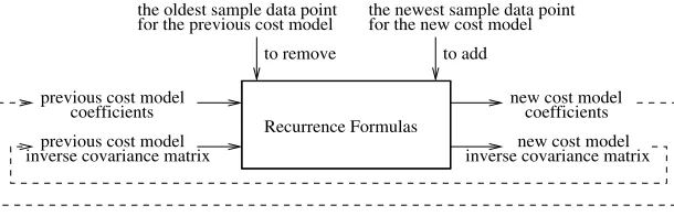
Fig. 3.The shifting method to evolve a cost model
The question now is if we can update the cost model more efficiently. We will present two efficient techniques for solving the problem in the next two sections.
3 The shifting method
Assume that we have obtained the initial cost modelM(0)(at timetk−1) via multiple regression based on initialksample data points(y0, xT0),(y1, xT1), . . . ,(yk−1,xTk−1). At timetk,
when new sample data point(yk, xTk)is observed, we need to
get cost modelM(1)based onksample data points(y1, xT 1),
(y2, xT2), . . . ,(yk, xTk). Can we avoid rebuildingM(1) from
scratch? Yes we can.
We notice that there arek−1common sample data points, i.e.,(y1, xT
1), . . . ,(yk−1, xTk−1), on which both cost models
M(1) andM(0) are based. This fact implies thatM(1) and
M(0)have a certain coherent relationship. Based on this servation, in this section we develop a shifting method to ob-tain new cost modelM(1)by adjusting old cost modelM(0). The basic idea is to add the effect of the newest sample data point(yk, xTk)toM(0)and in the meantime remove the effect
of the oldest sample data point(y0, xT
0)fromM(0), resulting in new cost modelM(1). That is,M(1)is obtained by shifting
M(0)one sample data point toward the new time.
Note that during the initial regression analysis forM(0)
we can get both the coefficients vectorβ(0) and the inverse covariance matrix[P(0)]−1(see Eq. 3). In the following dis-cussion, we assume that a cost model includes both the coeffi-cients vector and the inverse covariance matrix. Usingβ(0)and
[P(0)]−1for initial cost modelM(0)(together with(y 0, xT0) and(yk, xTk)), we can derive recurrence formulas to
calcu-lateβ(1) and[P(1)]−1 for new cost model M(1).β(1) and
[P(1)]−1can then be used to calculateβ(2)and[P(2)]−1for even newer cost modelM(2). In general, a new cost model
M(s)(s= 1,2, . . .) can be obtained by adjusting the previous cost modelM(s−1)(Fig. 3). Hence the cost model can evolve
smoothly over time with the dynamic environment in this way. A recurrence formula to update the cost model coefficients is given in the following theorem.
Theorem 1 The coefficientsβ(s)of new cost modelM(s)can
be recursively calculated by adjusting the coefficientsβ(s−1)
of previous cost modelM(s−1)(s= 1,2, . . .) as follows:
β(s)=β(s−1)+w(e/(1 +a)) +
w{e−xTs−1w(e/(1 +a))}/(1 +a) (5)
where
e=ys+k−1−xTs+k−1β(s−1), w= [P(s−1)]−1xs+k−1
a=xTs+k−1w, e =ys−1−xTs−1β(s−1)
w=−[P(s−1)]−1xs−1+
(wx Ts+k−1[P(s−1)]−1)xs−1/(1 +a)
a=xTs−1w
Proof.See Appendix.
Theorem 1 states that the coefficients β(s) of new model M(s) can be obtained by adjusting the coeffi-cients β(s−1) of previous model M(s−1). The adjustments
for the previous coefficients depend on the newest sam-ple data point ((ys+k−1, xT
s+k−1)), the oldest sample data
point ((ys−1, xTs−1)), the previous inverse covariance matrix
([P(s−1)]−1), and the errors (e ande) of using the previous
model to estimate query costs at the newest and oldest sample data points, which in turn depend on the previous coefficients (β(s−1)). Hence, the new coefficients can be obtained by
us-ing(ys+k−1, xTs+k−1),(ys−1, xTs−1),[P(s−1)]−1, andβ(s−1).
Note that β(s) obtained from Eq. 5 is the same as the one
obtained from the rebuilding approach in terms of accuracy. To use Eq. 5 to update the cost model iteratively for each new sample data point, we need not only the previous coef-ficients but also the previous inverse covariance matrix. Thus we also need to keep the inverse covariance matrix updated at each step. The following theorem gives the recurrence formula for updating the inverse covariance matrix.
Theorem 2 The inverse covariance matrix[P(s)]−1 of new
cost modelM(s)can be recursively calculated based on the
inverse covariance matrix[P(s−1)]−1of previous cost model
M(s−1)(s= 1,2, . . .) as follows:
[P(s)]−1= [P(s−1)]−1−
(wx Ts+k−1[P(s−1)]−1)/(1 +a)−wxTs−1{[P(s−1)]−1
−(wx Ts+k−1[P(s−1)]−1)/(1 +a)}/(1 +a) (6)
where
w= [P(s−1)]−1xs+k−1, a=xTs+k−1w
w=−[P(s−1)]−1xs−1+
(wx Ts+k−1[P(s−1)]−1)xs−1/(1 +a)
a=xTs−1w
Proof.See Appendix.
Equations 5 and 6 share many common factors. They can be evaluated efficiently by one algorithm. To further improve efficiency, the following formula
β(s)=β(s−1)+w(e/(1 +a)) +w[ys−1−xsT−1(β(s−1)
+w(e/(1 +a)))]/(1 +a) (7)
which is equivalent to Eq. 5, is adopted. The following al-gorithm updates the coefficients and the inverse covariance matrix of a cost model using the shifting method:
Algorithm 1 Cost model evolution based on the shifting
method.
Input: (1) Coefficients β(s−1) of previous model M(s−1);
(2) inverse covariance matrix[P(s−1)]−1 of previous model
M(s−1); (3) newest sample data point(y
s+k−1, xTs+k−1); (4) oldest sample data point(ys−1, xTs−1).
Output: (1) Coefficientsβ(s)of new modelM(s); (2) inverse
covariance matrix[P(s)]−1of new modelM(s).
Method:
1. Computew := [P(s−1)]−1x
s+k−1
2. Computea:=xT
s+k−1w;
3. ComputeuT :=xT
s+k−1[P(s−1)]−1
4. ComputeB:=wu T 5. ComputeA:=B/(1 +a)
6. ComputeC:= [P(s−1)]−1−A
/*first two terms in Eq. 6*/ 7. Computew:=C(−xs−1) 8. Computea:=xT
s−1w
9. ComputevT := xTs−1C 10. ComputeD:=wvT
11. ComputeE:=D/(1 +a)/*third term in Eq. 6*/ 12. Compute[P(s)]−1:=C−E
/*new inverse covariance matrix*/ 13. Computeyˆs+k−1:=xsT+k−1β(s−1)
14. Computee:=ys+k−1−yˆs+k−1 15. Computeh:=e/(1 +a)
16. Computer:=h w
17. Computeq:=β(s−1)+r/*first two terms in Eq. 7*/
18. Computeyˆs−1:=xTs−1q
19. Computeb:=ys−1−yˆs−1 20. Computed:=b/(1 +a)
21. Computeh:=d w/* third term in Eq. 7 */ 22. Computeβ(s):=q+h/* new coefficients*/
23. Returnβ(s)and[P(s)]−1
Starting with the initial cost modelM(0), Algorithm 1 can be repeatedly applied for each new sample data point to evolve the cost model for capturing the dynamic environment. The complexity of Algorithm 1 is given in the following corollary.
Corollary 1 Algorithm 1 requires8(n+ 1)2+ 7(n+ 1) + 2
number of scalar multiplications and divisions to calculate
β(s)and[P(s)]−1for new cost modelM(s)based onβ(s−1)
and[P(s−1)]−1of previous cost modelM(s−1), wherenis the
number of explanatory variables in the cost model.
Proof.Correctness can be easily checked by counting the num-ber of scalar multiplications and divisions required by each
step in Algorithm 1.
From Corollary 1, we can see that the asymptotic perfor-mance behavior of the shifting method for one step isθ(n2)
rather thanθ(n3)as required by the rebuilding approach via multiple regression for one step (Eq.4).
Another very attractive advantage of the shifting method is that its complexity is independent of sample sizek. To achieve a better cost model, the rebuilding approach has to employ a larger sample size, which implies a larger overhead, while the shifting method can obtain the same cost model without increasing any overhead. The reason for this phenomenon is that, no matter how large the sample set is, the difference between a new cost model and its previous cost model is only two sample data points, and the shifting method fully exploits the shared work for building two cost models based on the common sample data points rather than building the new cost model from scratch.
Furthermore, based on the fact thatk ≥ 10(n+ 2)(see footnote 2), we can show that the shifting method for one step is always more efficient than the rebuilding approach for one step for anyn ≥0. Clearly, the more steps the shifting method and the rebuilding approach are applied for, the more performance gain the shifting method will achieve. Therefore, we have the following important conclusion:
Corollary 2 The shifting method is more efficient than the
direct rebuilding approach for evolving a cost model in a dy-namic environment.
4 The block-moving method
The shifting method adjusts the cost model every time a new sample data point is observed. The cost model is kept up-to-date in this way. However, if the environment changes very slowly, people may want to accumulate several sample data points and use them to update the cost model all at once to re-duce the updating overhead. On the other hand, people some-times may want to run several sample queries in the current environment and use their observed data to update the cost model to capture the environment. In either case, we need to update the cost model based on a batch/block of sample data points rather than one individual sample data point.
Clearly, the block size should never be larger than the given sample size. If the block size equals the sample size, we can simply employ the rebuilding approach to update the cost model. If the block size is less than the sample size, as with the shifting method, we can derive recurrence formulas to calculate a new cost model based on its previous cost model for each block of sample data points observed.
Assume that we have cost model M(s−1) (includ-ing its coefficients β(s−1) and inverse covariance matrix
[P(s−1)]−1) at time t
s+k−2 (s = 1,2, . . .) based on k
sample data points (ys−1, xTs−1), (ys, xTs), . . . , (ys+k−2,
xT
s+k−2). At time ts+k+m−2, we want to obtain new cost modelM(s+m−1)based onk sample data points(y
s+m−1,
xT
s+m−1),(ys+m, xTs+m),. . . , (ys+k+m−2, xTs+k+m−2). Un-less block sizem=k, there are some common sample data points(ys+m−1, xT
s+m−1), . . . ,(ys+k−2, xTs+k−2)(1≤m <
inverse covariance matrix[P(s+m−1)]−1for new cost model
M(s+m−1)based on (1) the previous coefficientsβ(s−1); (2)
the previous inverse covariance matrix [P(s−1)]−1; (3) the
newest block of sample data points (ys+k−1, xTs+k−1), . . . ,
(ys+k+m−2, xTs+k+m−2); and (4) the oldest block of sample
data points(ys−1, xTs−1), . . . ,(ys+m−2, xTs+m−2).
Figure 3 can still illustrate the idea of this method, except that (1) the newest sample data point should be replaced by the newest block of sample data points and (2) the oldest sample data point should be replaced by the oldest block of sample data points. Since this method updates the cost model for each new block of sample data points instead of each individual new sample data point, we call this method the block-moving method.
The following theorem specifies the recurrence formula for updating the coefficients of the cost model.
Theorem 3 The coefficients β(s+m−1) of new cost model
M(s+m−1)can be recursively calculated by adjusting the
co-efficientsβ(s−1)of previous cost modelM(s−1)(s= 1,2, . . .)
as follows:
β(s+m−1)=
(I−H Prem)−1(I+ [P(s−1)]−1Padd)−1β(s−1)+
(I−H Prem)−1H(b
add−brem) (8)
where
Padd=
s+k+m−2
i=s+k−1
xixTi, Prem=
s+m−2
i=s−1
xixTi
badd=
s+k+m−2
i=s+k−1
xiyi, brem=
s+m−2
i=s−1
xiyi
H= (I+ [P(s−1)]−1Padd)−1[P(s−1)]−1
andIis the(n+ 1)×(n+ 1)identity matrix.
Proof.See Appendix.
As with the shifting method, to apply the block-moving method we also need to keep the inverse covariance matrix updated for each block. The following theorem specifies the recurrence formula for updating the inverse covariance matrix of the cost model.
Theorem 4 The inverse covariance matrix[P(s+m−1)]−1of
new cost model M(s+m−1) can be recursively calculated based on the inverse covariance matrix[P(s−1)]−1 of
pre-vious cost modelM(s−1)(s= 1,2, . . .) as follows: [P(s+m−1)]−1=
{I−((I+ [P(s−1)]−1Padd)−1[P(s−1)]−1)Prem}−1
(I+ [P(s−1)]−1P
add)−1[P(s−1)]−1 (9)
where
Padd=
s+k+m−2
i=s+k−1
xixTi, Prem=
s+m−2
i=s−1
xixTi
andIis the(n+ 1)×(n+ 1)identity matrix.
Proof.See Appendix.
Since Eqs. 8 and 9 share some common terms, the fol-lowing algorithm efficiently updates both the coefficients and the inverse covariance matrix of a cost model using the block-moving method:
Algorithm 2 Cost model evolution based on the
block-moving method.
Input: (1) Coefficients β(s−1) of previous modelM(s−1);
(2) inverse covariance matrix[P(s−1)]−1 of previous model
M(s−1); (3) newest block of sample data points (ys+k−1,
xT
s+k−1), . . . ,(ys+k+m−2,xTs+k+m−2); (4) oldest block of
sample data points(ys−1, xTs−1), . . . ,(ys+m−2, xTs+m−2). Output: (1) Coefficientsβ(s+m−1)of new modelM(s+m−1);
(2) inverse covariance matrix [P(s+m−1)]−1 of new model
M(s+m−1).
Method:
1. ComputePadd=is=+sk++km−−12xixTi
2. ComputeF= [P(s−1)]−1Padd 3. ComputeG=I+F
4. ComputeG−1
5. ComputeH=G−1[P(s−1)]−1
6. ComputePrem=is=+sm−−12xixTi
7. ComputeJ=HPrem 8. ComputeK=I−J 9. ComputeK−1
10. Compute[P(s+m−1)]−1=K−1H /*new covariance from Eq. 9*/ 11. Computeo=G−1β(s−1)
12. Computem =K−1o; /*first term in Eq. 8*/ 13. Computebadd=
s+k+m−2
i=s+k−1 xiyi
14. Computebrem=
s+m−2
i=s−1 xiyi
15. Computedone=badd−brem
16. Computen= [P(s+m−1)]−1d one
/*second term in Eq. 8*/
17. Computeβ(s+m−1)=m +n; /*from Eq. 8*/
18. Returnβ(s+m−1)and[P(s+m−1)]−1
Starting with the initial cost model M(0), Algorithm 2 can be repeatedly applied for each new block of sample data points to evolve the cost model for capturing the dynamic environment. The complexity of Algorithm 2 is given in the following corollary.
Corollary 3 Algorithm 2 requires6(n+ 1)3+ (2m+ 3)(n+
1)2+2m(n+1)number of scalar multiplications and divisions
to calculateβ(s+m−1)and[P(s+m−1)]−1for new cost model
M(s+m−1)based onβ(s−1)and[P(s−1)]−1of previous cost
modelM(s−1), wherenis the number of explanatory variables in the cost model andmis the block size.
Proof.Correctness can be easily checked by counting the num-ber of scalar multiplications and divisions required by each
step in Algorithm 2.
Note that the complexity of Algorithm 2 depends not only on the numbernof explanatory variables but also the block sizem(≤k). If block sizemis very close to the sample size
mis relatively small compared with sample sizek. The fol-lowing corollary specifies a condition for the block-moving method to be superior.
Corollary 4 The block-moving method is more efficient than
the rebuilding approach if and only if block size m <
1/2[−5(n + 1) + (k + 3) − 1/(n + 2)]. For the mini-mal sample sizek = 10∗(n+ 2), the condition becomes m <1/2[5(n+ 1) + 13−1/(n+ 2)].
Proof.The claims follow from Eq. 4 and Corollary 3. Lengthy algebraic derivations are omitted.
Note that the block size determines how many steps we want to combine in the procedure for evolving the cost model. The larger the block size, the more evolutionary overhead is reduced. To obtain a quality cost model, one usually uses a sample with a large size (much larger than the minimal one). This allows a large block size to be used for the block-moving method. However, a large block size may cause the evolution of the cost model to be not smooth. Thus a fixed number (e.g., 10) that is much smaller than the sample size is usually chosen as the block size for the block-moving method. As with the shifting method, the performance of the block-moving method is independent of the sample size, but it guarantees the same quality of the cost model produced by the rebuilding approach with a large sample.
Comparing the block-moving method with the shifting method, it is not difficult to see from Corollaries 1 and 3 that applying the shifting method once is more efficient than apply-ing the block-movapply-ing method once for block sizem >1. This is because the latter needs to take more new sample data points into consideration for updating the cost model. However, to obtain the same modelM(s+m−1)from old modelM(s−1),
the shifting method has to be appliedmtimes, while the block-moving method only needs to be applied once. Hence the com-plexity for obtainingM(s+m−1)fromM(s−1)via the shifting
method is:
8m(n+ 1)2+ 7m(n+ 1) + 2m (10)
Comparing Eq. 10 with Corollary 3, we notice that the block-moving method is more efficient whenmis sufficiently large, while the (repeated) shifting method is more efficient when
mis very small. The following corollary gives a condition for each method to be superior.
Corollary 5 Whenm ≥ (n+ 1), the block-moving method
is more efficient than the shifting method. Whenm <3(n+
1)2/(5n+ 7), the shifting method is more efficient than the
block-moving method.
Proof.The claims follow from Eq. 10 and Corollary 3. Lengthy algebraic derivations are omitted.
Note that Corollary 4 gives a sufficient and necessary con-dition, while Corollary 5 gives two sufficient conditions only. From Corollaries 4 and 5, we know that block size m
cannot be too small (e.g.,m≥(n+1)) in order for the block-moving method to outperform the shifting method, and block sizemcannot be too large (i.e.,m < 1/2[5(n+ 1) + 13−
1/(n+ 2)]) in order for the block-moving method to outper-form the rebuilding approach. Clearly we have the following conclusion:
Application m Application 2
Application 1
DB DB
DB
DBMS DBMS
DBMS
MDBS Agent MDBS Agent
MDBS Agent
Local DBS 2
Local DBS 1 Local DBS n Local Local Local
[image:7.595.310.553.50.193.2]Local Local Local MDBS Global Server
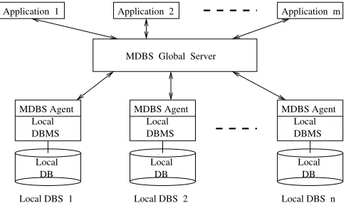
Fig. 4.A multidatabase system architecture
Corollary 6 For an appropriately chosen block size, the
block-moving method can be superior to both the rebuilding approach and the shifting method in terms of time efficiency.
Be aware that some intermediate cost models are skipped if the block-moving method is applied compared with the shifting method. Therefore, the latter is still a better choice if smooth evolution and accuracy are desired.
5 Implementation considerations
The cost model evolution techniques discussed in the previ-ous sections were developed for a multidatabase environment running the multidatabase prototype CORDS-MDBS [2].
Figure 4 shows the system architecture for CORDS-MDBS. In CORDS-MDBS, the global data model is assumed to be relational and each local DBS is associated with an MDBS agent that provides a relational interface if the local DBMS is nonrelational. Thus the global query optimizer in the MDBS may view participating local DBMSs as relational ones. Note that the cost model evolution techniques suggested in this paper do not rely on the relational data model. As long as a query class and the explanatory variables of its cost model are identified, the techniques can be applied directly to evolve the cost model even if the data model is nonrelational.
to evolve the relevant cost model via the chosen evolutionary technique.
One potential problem that needs to be considered here is the starvation problem. It is possible that user queries for a particular query class are not executed as frequently as re-quired to capture the dynamic environment. If user queries for a query class are in fact never used in an application en-vironment, the solution is simple – we can simply ignore the update of the corresponding cost model since we only need to maintain those cost models that are useful for practical user queries. However, if the query class is indeed needed in appli-cations but its queries are not run as often as the environment changes, one solution in this case is to generate and run some additional artificial sample queries when necessary to supple-ment the user sample queries. The system makes full use of user queries and also keeps the cost model up-to-date, although some extra overhead cannot be avoided in this case.
The opposite of the starvation problem is the overflow problem. In other words, user queries are executed too fre-quently for a particular query class. In this case, the employed evolutionary technique should not take every user query as a sample query to update the cost model because there might be very little change in the underlying environment since the last update. One solution to this problem is to periodically pick up a user query as a sample query to evolve the cost model. Another solution is to activate the cost model updating pro-cedure whenever an observable change in the environment is detected (e.g., the number of queries with a large error of cost estimation is beyond a threshold) and to deactivate the cost model updating procedure when the cost model is up-to-date. In a practical system, the evolution procedure can also be con-trolled manually via some system configuration parameters or system commands.
As pointed out previously, the evolutionary techniques de-veloped in this paper are suitable for capturing the effect of the slowly changing factors on a cost model in a dynamic en-vironment. These factors usually change little by little (i.e., do not cause an abrupt dramatic change to the underlying system environment at any time). However, a significant environmen-tal change may be accumulated after a certain period of time (e.g., a couple of days, weeks, or months). We need to keep the cost model updated as the environment changes. If the environmental change exceeds a certain level when the next sample data point is obtained, the shifting method should be employed to update the cost model using the new sample data point. Otherwise, the newly observed sample data point is kept in a block (set) to be used by the block-moving method for updating the cost model at a later time. Note that if the environ-mental change is too small (negligible) when the next sample data point is obtained, this sample data point can be skipped since it has little effect on the cost model (notice that if the environment changes very slowly, we do not need to update the cost model often). Hence we assume that the next sample data point is obtained when the underlying environment ex-periences an observable (nonnegligible) change since the last sample data point.
In fact, the shifting method and the block-moving method can be applied together in the following integrated scheme to evolve a cost model for a slowly changing environment. LetM
be the current cost model andQi, Qi+1, . . .be the incoming sequence of sample queries. Letε(Qj)be the relative error of
the estimated cost given by current cost modelM for sample queryQj(j =i, i+ 1, . . .). A large estimation error usually
indicates that the cost model needs to be updated to reflect the environmental change. Hence ifε(Qi)is greater than or equal to a thresholdd1(e.g., 70%, which can be calibrated through experiments), we apply the shifting method to update cost modelM using the sample data point forQi. Ifε(Qi)is
less than thresholdd1, the sample data point forQiis kept as
one of the sample data points in the block to be used by the block-moving method for the next update of the cost model. The subsequent errorsε(Qi+1),ε(Qi+2), . . .ε(Qi+(m−1))are
examined until either (1)ε(Qi+(m−1))is larger than threshold
d1or (2) the numbermof kept sample data points reaches a block size chosen based on Corollaries 4 and 5. The block-moving method is then applied to update current cost model
Musing the block ofmsample data points for sample queries
Qi,Qi+1, . . .Qi+(m−1). Note that if the numbermof kept
sample data points is too small in case (1), to improve the performance (see Corollary 5), the shifting method (rather than the block-moving method) could be repeatedly applied to each sample data point in the block to achieve the same final updated cost model. This integrated scheme aims to achieve both good efficiency and smoothness of a cost model evolution, taking advantage of both the shifting and block-moving methods.
Note that the rebuilding approach can always be applied to update a cost model. However, its efficiency is usually not as good as the evolutionary techniques. To reduce overhead, we cannot apply the rebuilding approach frequently. As a re-sult, the cost model may not change smoothly. Every time a cost model changes significantly, many compiled (optimized) queries may need to be reoptimized for the new environment, which causes the system to be jammed with reoptimization jobs. A smooth change of the cost model helps the job sched-uler to properly schedule reoptimization jobs so that a system jam is avoided. Hence the evolutionary techniques are the ef-ficient and seamless approaches to evolving cost models in a slowly changing environment.
However, there are cases for which the evolutionary tech-niques are not Suitable, for example, if the environment stays unchanged for a long time (e.g., many months/years) and then suddenly experiences a dramatic change (e.g., caused by hard-ware or softhard-ware upgrade). The evolutionary techniques are no longer applicable since all previous sample data points be-come useless and a new set of sample data points are needed to establish the new cost model. The monolithic rebuilding approach can be applied in such a case. On the other hand, if the environment changes very rapidly (e.g., within a few seconds, minutes, or hours), the evolutionary techniques are not applicable either since an evolutionary cost model may not be stable. Special techniques such as the qualitative approach [19], the fractional analysis approach [20], and the probabilis-tic approach [20] are needed to solve query cost estimation issues in such an environment. Besides, the conventional dy-namic query optimization techniques could also be adopted in such a case.
updates are done on the fly, the overhead of such a technique is required to be as small as possible. So far no technique has been proposed to automatically adjust the parameters of a cost model in such a system. Our techniques in this paper can be utilized to solve this issue in such systems.
6 Experimental results
To examine the effectiveness and efficiency of the evolution-ary techniques discussed in the previous sections, we con-ducted extensive experiments in our multidatabase environ-ment, where Oracle 8.0 and DB2 5.0 were used as local DBMSs running under SunOS 5.1 on SUN UltraSparc 2 work-stations.
Note that conducting extensive experiments in a real slowly changing environment is infeasible since it would take too long to complete the experiments. To effectively simulate a slowly changing dynamic environment, we artificially gen-erated different numbers of concurrent processes with various work/sleep ratios to change the system contention level in a given environment. The cost of a small probing query is used to gauge the system contention level. The higher the probing query cost, the higher the system contention level. Forty-nine system contention levels (with the probing query cost ranging from 3 seconds to 98 seconds) were considered in both the Or-acle and DB2 environments. A slowly changing environment was achieved by assuming that the system contention level gradually changes from the lowest level 1 to the highest level 49. Note that we basically adjusted the frequently changing factors (i.e., CPU load, memory usage, etc.), which are easy to manipulate, to change the environment and kept each change stable for some time to simulate a slowly changing environ-ment. The essentials of our evolutionary techniques are their capability to evolve a cost model to capture the environmen-tal change (reflected in the updated coefficients), no matter what causes the environment to change. The main purpose of our experiments is to verify the evolution capabilities of the techniques. Hence the above simulated environments are reasonable for the experiments.
The experimental databases used in the experiments were the same as those in [19–21]. More specifically, each lo-cal database consists of 12 tables Ri(a1, a2, . . . , aj) (i =
1,2, . . . ,12;j∈ {3,5,7,9,11,13}) with data randomly gen-erated and cardinalities ranging from 3,000∼250,000. Each table has a number of indexed columns and various selectivi-ties for different columns.
Note that our evolutionary techniques do not rely on any particular query class. The experimental results for all query classes are similar. In this section, we report typical experi-mental results for a representative query classG15(defined in [21]) consisting of unary queries that have no usable indexes in their qualification conditions. To demonstrate that the tech-niques have a similar behavior for other query classes, we also report some experimental results for another query classG14 consisting of unary queries that have usable (nonclustered) indexes in their qualification conditions.
The sample queries used to evolve cost models were ran-domly chosen from the relevant query class. One hundred sam-ple queries were executed at each system contention level on both Oracle 8.0 and DB2 5.0. Hence a total of 4900 sample
queries were executed in a sequence for each environment. The first 100 sample queries (i.e., sample sizek= 100) were used to derive the initial cost model (withn = 6variables, i.e., the cardinality of the operand table, the cardinality of the result table, the tuple length of the operand table, the tuple length of the result table, the physical size of the intermediate table, and the physical size of the operand table [21]) via the query sampling method. The effect of environmental factors, such as physical data distribution and system buffer setup, on query performance is reflected in the coefficients of the vari-ables in the cost model. The evolutionary techniques were then used to evolve the cost model (i.e., updating the coefficients) to capture the dynamic environment. The shifting method was used to adjust the cost model every time a new sample query point was observed from the execution sequence, while the block-moving method was used to adjust the cost model ev-ery time a block of sample quev-ery points was observed from the execution sequence.
To examine the accuracy of the evolutionary cost mod-els obtained from the evolutionary techniques, we also ran some test queries randomly chosen from the query class in both the Oracle and DB2 environments. The cost of each test query was estimated by using the corresponding updated cost model in the environment, and the observed and estimated costs were compared. To see accuracy gains from the evolu-tion techniques, the cost estimates using the initial (static) cost model were also compared.
Note that, unlike scientific computation in engineering, the accuracy of cost estimation in query optimization is not required to be very high. In analysis on the experiments, the cost estimates with relative errors within 30% are considered to be very good, and the cost estimates that are within the range of one-time larger or smaller than the corresponding observed costs (e.g., 2 min vs. 4 min) are considered to be good. Only those cost estimates that are not of the same order of magnitude with the observed costs (e.g., 2 min vs. 3 h) are not acceptable. Table 1 shows the percentages of good and very good cost estimates for test queries inG15 at four representative contention levels (each level has 100 test queries) on Oracle 8.0 and DB2 5.0. In the table, cost estimates from the initial (static) cost model, the evolutionary cost model by the shifting method, and the evolutionary cost model by the block-moving method (m= 10) were listed. To show that the experimental results are similar for different query classes, Table 2 lists two representative sets of experimental results for another query classG14.
From the experiments, we have the following observations on the effectiveness of the evolutionary techniques:
Table 1.Percentages of good cost estimates for test queries inG15from experiments on Oracle 8.0 and DB2 5.0 Local Contention Static: Static: Shifting: Shifting: Block-moving: Block-moving:
DBMS level very good% good% very good% good% very good% good%
12 1% 5% 83% 88% 78% 87%
Oracle 25 0% 0% 70% 82% 68% 79%
37 1% 3% 63% 74% 59% 74%
49 0% 1% 70% 87% 68% 78%
12 0% 1% 85% 93% 85% 90%
DB2 25 0% 0% 82% 91% 78% 87%
37 0% 0% 65% 88% 53% 73%
49 0% 0% 90% 97% 93% 97%
[image:10.595.45.451.246.298.2]Average 0.25% 1.25% 76% 87.50% 72.75% 83.13%
Table 2.Similar experimental results obtained for test queries inG14on Oracle 8.0
Local Contention Static: Static: Shifting: Shifting: Block-moving: Block-moving: DBMS level very good% good% very good% good% very good% good%
Oracle 12 0% 1% 82% 93% 81% 91%
25 1% 1% 86% 92% 78% 88%
2400 2410 2420 2430 2440 2450 2460 2470 2480 2490 2500 −200
0 200 400 600 800 1000 1200
Query Number
Query Cost (Elapsed Time Units)
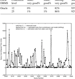
solid line (*) −− observed costs
dashed line (o) −− estimated costs from evolutionary cost model (shifting) dotted line (+) −− estimated costs from static cost model
Fig. 5.Cost estimates for test queries inG15from static and shifting models at contention level 25 on Oracle 8.0
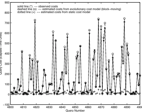
time measuring unit for the relevant commercial systems is not revealed here to avoid a potential license violation. • The block-moving method can also derive a good evolu-tionary cost model to capture a slowly changing dynamic environment. From Table 1 we can see that the evolution-ary cost model obtained from the block-moving method can give good cost estimates for most test queries (83.13% on average, including 72.75% very good ones), which is much better than the initial static cost model. Figures 7 and 8 show a typical comparison for cost estimates from the two cost models in Oracle 8.0 and DB2 5.0, respec-tively. Comparing the shifting and block-moving meth-ods, a cost model obtained from the former is more accu-rate than the one obtained from the latter, as pointed out in Sect. 4. In general, the more rapidly the environment
2400 2410 2420 2430 2440 2450 2460 2470 2480 2490 2500 −200
0 200 400 600 800 1000
Query Number
Query Cost (Elapsed Time Units)
solid line (*) −− observed costs
[image:10.595.45.296.252.515.2]dashed line (o) −− estimated costs from evolutionary cost model (shifting) dotted line (+) −− estimated costs from static cost model
Fig. 6.Cost estimates for test queries inG15from static and shifting models at contention level 25 on DB2 5.0
changes and the larger the block size, the better accuracy can be obtained by the shifting method over the block-moving method.
[image:10.595.307.550.325.513.2]shift-4800 4810 4820 4830 4840 4850 4860 4870 4880 4890 4900 −200
0 200 400 600 800 1000 1200 1400 1600
Query Number
Query Cost (Elapsed Time Units)
solid line (*) −− observed costs
[image:11.595.47.289.48.237.2]dashed line (o) −− estimated costs from evolutionary cost model (block−moving) dotted line (+) −− estimated costs from static cost model
Fig. 7.Cost estimates for test queries inG15from static and block-moving models at contention level 49 on Oracle 8.0
4800 4810 4820 4830 4840 4850 4860 4870 4880 4890 4900 −100
0 100 200 300 400 500 600 700 800 900
Query Number
Query Cost (Elapsed Time Units)
solid line (*) −− observed costs
[image:11.595.307.551.51.242.2]dashed line (o) −− estimated costs from evolutionary cost model (block−moving) dotted line (+) −− estimated costs from static cost model
Fig. 8.Cost estimates for test queries inG15from static and block-moving models at contention level 49 on DB2 5.0
ing method. From the figure we can see that the relative errors become larger and larger for the static cost model as the environment moves farther and farther away from the initial one, while the relative errors are kept within 30% by the evolutionary cost model no matter how much the environment changes.
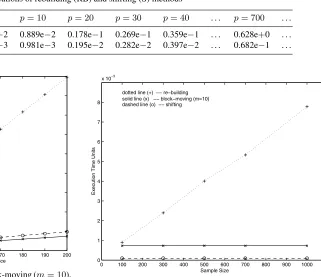
To examine the efficiency of the evolutionary techniques, we compared the execution costs of the shifting method, the block-moving method, and the rebuilding approach for var-ious cases. Table 3 shows the execution time units for one invocation (step) of each technique. Table 4 shows the execu-tion time units for repeated invocaexecu-tions (multiple steps) of the shifting method and the rebuilding approach, wherepis the number of times the relevant method is invoked to update the cost model forpconsecutive new sample data points. Note that the block-moving method is invoked only once for each block of sample data points rather than for each individual point.
0 5 10 15 20 25 30 35 40 45 50 −0.4
−0.2 0 0.2 0.4 0.6 0.8 1
Contention Level
Relative Error
solid line −− relative errors from the static cost model
dashed line −− relative errors from the evolutionary cost model (shifting)
Fig. 9.Errors for cost estimates of a query executed at various con-tention levels from static and evolutionary (shifting) cost models on Oracle 8.0
Hence it is not compared in Table 4. From the experiments, we have the following observations on the efficiency of the evolutionary techniques:
• The shifting method is more efficient than the rebuilding approach, as predicated by Corollary 2 from theoretical analysis. Table 4 indicates that the former can improve efficiency by about 89% for anyp, i.e., the cost of the re-building approach is about eight times larger than that of the shifting method. The more times (steps) the shifting method is invoked, the more (absolute) overhead can be saved (Fig. 10). Note that the sample size (i.e., 100) used in the experiments was close to the minimum (i.e., 80) for the given query class. The above performance improve-ment is mainly caused by the complexity reduction from
θ(n3)toθ(n2). On the other hand, to improve the qual-ity of a regression cost model, one ought to use a sample with a larger sizek. Given that the query class for which the cost model was developed contains a large number of queries [21], a sample of 1000 or more queries could be used. However, as pointed out earlier, the cost of the shift-ing method is independent of sample sizek, while the cost of the rebuilding approach is proportional tok(Fig. 11). In fact, for a sample of size 1000, the cost of the latter is about 77 times larger than that of the former (to obtain the same result). Furthermore, the query class considered in the experiments was relatively simple. For a more com-plex query class (e.g., a join query class [21]), both the numbernof explanatory variables and the sample sizek
(increasing withn, as indicated in footnote 2) can be much larger. The overhead saving by the shifting method can be even more significant.
• The efficiency of the block-moving method depends on the block size. The larger the block size, the higher the execu-tion cost.
− When the block size is relatively small (e.g., m =
[image:11.595.48.287.288.476.2]Table 3.Execution time units for one-step rebuilding, shifting, and block-moving methods
Method RB S BM (3) BM (5) BM (10) BM (20) BM (30) BM (40) . . .
One-step
[image:12.595.218.539.151.428.2]execution cost 0.904e−3 0.110e−3 0.631e−3 0.680e−3 0.775e−3 0.973e−3 0.117e−2 0.151e−2 . . . RB – rebuilding method; S – shifting method; BM (m) – block-moving method with block sizem
Table 4.Execution time units for repeated invocations of rebuilding (RB) and shifting (S) methods
Repeat#p p= 1 p= 3 p= 5 p= 10 p= 20 p= 30 p= 40 . . . p= 700 . . . RB 0.904e−3 0.268e−2 0.445e−2 0.889e−2 0.178e−1 0.269e−1 0.359e−1 . . . 0.628e+0 . . . S 0.110e−3 0.305e−3 0.498e−3 0.981e−3 0.195e−2 0.282e−2 0.397e−2 . . . 0.682e−1 . . .
100 110 120 130 140 150 160 170 180 190 200 0
0.01 0.02 0.03 0.04 0.05 0.06 0.07 0.08 0.09
Sample Data Point Number in the Sequence
Execution Time Units
[image:12.595.52.357.158.421.2]dotted line (+) −− re−building (repeated for every point) dashed line (o) −− shifting (repeated for every point) solid line (x) −− block−moving (repeated for every block, m=10)
Fig. 10.Efficiency comparison for shifting, block-moving (m= 10), and rebuilding methods
once (Table 3). The former can improve efficiency as much as 52% in such a case. If the rebuilding approach is invoked multiple times to keep the cost model up-to-date for each new sample data point, the perfor-mance gain from the block-moving method can be even dramatically larger. The block-moving method becomes inefficient, compared to the (one-step) re-building approach, if the block size is relatively large (e.g.,m= 30in Table 3). In such a case, the latter can be used efficiently to keep the cost model up-to-date for each block of sample data points rather than the former. However, the cost of the rebuilding approach increases with sample size k, while the cost of the block-moving method is independent ofk (Fig. 11). Increasing the sample size (either to improve the cost model quality or to handle a more complex query class) would make the rebuilding approach less efficient than the block-moving method with a larger block size. − When block sizemis not too small (e.g., m = 10),
invoking the block-moving method once is more ef-ficient than the (repeated) shifting method, which has to be invoked multiple times to keep the cost model up-to-date for every sample data point (including the sample data point at the end of each block). The
per-0 100 200 300 400 500 600 700 800 900 1000 1100 0
1 2 3 4 5 6 7 8
x 10−3
Sample Size
Execution Time Units
dotted line (+) −− re−building solid line (x) −− block−moving (m=10) dashed line (o) −− shifting
Fig. 11.Performance effect of sample size on (one-step) rebuilding, shifting, and block-moving techniques
formance gain can be as much as 62%. Otherwise, the latter may be more efficient (e.g.,m= 3,5).
− There are cases (e.g.,m = 10) in which invoking the block-moving method once is more efficient than using either the (repeated) shifting method or the rebuilding approach (once). If all the methods are invoked re-peatedly to keep the cost model up-to-date in such a case, the block-moving method can save a significant amount of overhead over time (Fig. 10).
The observations on the block-moving method are consis-tent with Corollaries 4 to 6 from our theoretical analysis.
7 Conclusions
A major challenge for performing global query optimization in an MDBS is that the cost models for local DBSs may not be available at the global level. Dynamic environmental factors add more difficulties to this problem. In this paper, we have suggested evolving a cost model to capture a slowly changing dynamic multidatabase environment so that the cost model is kept as accurate as possible all the time.