Post-processing modeling and removal of background noise in space-based time-of-flight sensors
Daniel. J. Gershman,1 Jason A. Gilbert,1 Jim M. Raines,1 George Gloeckler,1 Patrick Tracy,1 and Thomas H. Zurbuchen1
Department of Atmospheric, Oceanic, and Space Sciences, University of Michigan,
Ann Arbor, MI, USA
This paper develops and implements a mathematical framework that enables noise
modeling and removal for any sensor that relies on discretely measured events. Here,
we apply this technique to data from the Fast Imaging Plasma Spectrometer (FIPS),
a time-of-flight mass spectrometer on the MESSENGER spacecraft. An iterative
Monte Carlo event-processing algorithm is used to probabilistically separate
instru-ment measureinstru-ments into real and noise-based events. Kernel density estimation is
employed as a smoothing technique to enable noise removal for datasets comprised
of only a few events. Given an accurate noise model, the overall misidentification of
events is expected to be less than 25% even for datasets having low signal-to-noise
(SNR) ratios, with substantially improved results expected for progressively larger
accumulations of data. These techniques are shown to successfully recover heavy ion
events from in-flight FIPS data both inside and outside Mercury’s magnetosphere.
Such data analysis methods not only drive a more in-depth understanding of sensor
operation, but also provide a unique post-processing approach that can result in the
improvement of in-flight SNR without any modifications to instrument settings. In
addition, these method are readily applicable to existing archived datasets of past
I. INTRODUCTION
Noise events in a spaceborne time-of-flight mass spectrometer (TOF-MS) are undesirable
measurements that can arise from a variety of sources, ranging from background processes
to incident particle events. These erroneous events contaminate mass and energy spectra,
making it difficult to recover accurate ion composition and abundances, especially for heavy
ion species for which measured event rates can be low. A number of these noise sources, as
well as their effects on data analysis are introduced and discussed in detail by Gilbert et al.1.
Here, we focus on modeling and probabilistic removal of these events, such that the
signal-to-noise ratio (SNR) of measured datasets can be increased using software post-processing
techniques rather than adjusting limited in-flight instrument settings. The techniques
de-scribed here were used to enable a number of scientific analyses2–5 of observations from the
Fast Imaging Plasma Spectrometer (FIPS)6,7 on the MErcury Surface, Space ENvironment,
GEochemistry, and Ranging (MESSENGER) spacecraft8, currently in orbit around Mercury.
There are two general classes of noise contamination: additive and multiplicative/distortion.
Additive noise is an unwanted signature superimposed on top of a real signal9. The most
common and perhaps ubiquitous form of this contamination is white noise10, with a constant
spectral density and a Gaussian distribution of amplitudes typically superimposed on an
audio, electronic, or image signal. For any additive noise source, however, the underlying
signal remains unchanged. Distortion, on the other hand, involves a convolution of the
uncontaminated signal with a noise function, altering its original properties11. A simple
example of distortion is image blurring, whereby the color in a particular pixel is changed
on the basis of the original properties of its neighbors12.
The vast majority of noise events in a TOF-MS are additive. Although, as will be
discussed, the intensity of some noise sources will scale with the number of real events, these
noise events are nonetheless superimposed on the measured distribution of incident particles.
Therefore, TOF-MS noise removal typically requires only distribution separation rather than
dataset deconvolution. Also, the TOF-MS noise sources discussed here will be characterized
with accumulations of instrument data and will consequently be well-known. A known source
is considerably easier to remove from a dataset than an unknown one, and consequently we
will not require the use of complex blind-signal separation techniques13. Finally, the ability to
to the removal process, allowing each event to be analyzed individually and completely, as
opposed to being limited by the real-time processing power of an on-board flight computer.
In the case of many audio and image processing applications, noise sources exhibit specific
spectral signatures14. After a frequency analysis of a particular dataset, high- or low-pass
filtering can be used to reduce markedly the contribution of many noise sources15. This
strategy, however, may not be best suited for applications to TOF-MS measurements that
are a set of discrete, multi-dimensional events for which properties must not be altered
as a consequence of any noise reduction process. Instead, we will employ Monte Carlo
techniques16 to process instrument-measured events. Monte Carlo techniques have been
applied to a wide variety of applications in fields such as statistical physics17, biology18,
and finance19. Although these techniques vary in their implementation, they all use a set
of sampled random numbers to aid in their computations. Here, the probability that a
particular event is noise will be derived with an instrument-noise forward model. These
probabilities, in conjunction with randomly generated numbers will be used to process sets
of TOF-MS observations.
The primary obstacle for accurate noise reduction for TOF-MS data is low measured
event rates. TOF-MS measurements are discrete datasets that often result in zero recorded
events for a given time step, as opposed to an analog audio signal or a digital image. In
fact, most measured TOF-MS data will rarely form a smooth distribution function unless
they are accumulated over long time periods. The challenge here is to reconstruct a smooth
distribution function sufficient for event processing based on only a few discrete events.
Data from MESSENGER/FIPS are used as examples for both noise forward modeling
and removal processes. FIPS is a double-coincidence TOF-MS, composed of an electrostatic
analyzer (ESA) and a TOF section. As illustrated in Figure 1, charged particles are guided
by an electric field between shaped electrodes of the ESA such that only ions with a
par-ticular energy per charge (E/q) ratio successfully reach and penetrate a thin carbon foil,
liberating secondary electrons. These electrons are accelerated by electric fields in the TOF
section and electrostatically reflected by a mirror harp assembly onto a microchannel plate
(MCP) detector, where they create a start signal. The incident particle, which is most often
neutralized by the foil20, passes through the mirror harp assembly to another MCP detector,
generating a stop signal, resulting in a correlated TOF event. The anode in the start MCP
FIG. 1. Illustration of the MESSENGER/FIPS TOF-MS adapted from Andrews et al.7. Ions with
a particular range of E/q are filtered through an ESA and then analyzed by a TOF section with
imaging capabilities on the start detector. The yMCP coordinate direction of the MCP is out of
the plane of the figure.
per charge E/q, T OF, and start MCP coordinates (xMCP, yMCP), with coordinate system geometry defined in Figure 1.
Although FIPS is used as a case study, the techniques developed here should be readily
generalizable to any MS. In Section II, we develop a mathematical framework for
TOF-MS measurements as well as a noise removal process suitable for datasets with varying SNR
and low total count rates. In Section III, we discuss a method to create a complete
TOF-MS noise forward model from accumulations of measured data, using MESSENGER/FIPS
as an example. Finally, in Section IV, we apply the noise forward modeling and removal
processes to successfully recover measured heavy ion events in and around the magnetosphere
of Mercury from MESSENGER/FIPS in-flight observations.
II. MATHEMATICAL FRAMEWORK
In order to model noise in a TOF-MS sensor, a mathematical framework for describing
how an instrument measures events must be developed. Such a framework will enable
TABLE I. Notation used for the mathematical framework of TOF-MS noise modeling and removal
processes. Here, Φ is a dummy variable used to represent any of several different quantities and
distributions introduced throughout the paper.
Notation Definition
Φreal Real signal distribution of Φ
Φnoise Noise signal distribution of Φ
Φbg Background signal distribution of Φ
Φinc Incident particle signal distribution of Φ
ˆ
Φ Normalized distribution of Φ
Φm Φ derived from instrument measurement
Φ∗ Φ derived from noise-removal processing
are applicable to any TOF-MS. Table I introduces notation that is used to describe quantities
throughout the paper. Additional subscripts and superscripts that appear throughout the
paper but are not given in Table I will be defined at first use. The derivations here, as
well as the noise processing developed later in this section, are limited to one dimension.
However, as will be discussed, these results will apply to multi-dimensional datasets.
A. Measured events
Let the distribution of all measured events with respect to some parameter,x, be defined asfm(x). In general,xis one of the measurable event parameters (e.g.,t,E/q,T OF). Since it is produced from discretely measured events, fm(x) necessarily can only have integer values. The measured events that form fm(x) can be considered to be a set of random samples of some probability density distribution, f(x). f(x) can have non-integer values, but its total integrated value must be the same as forfm(x) such that, for all possible values of x,
X i
fm(xi) = X
i
f(xi). (1)
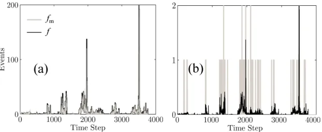
FIG. 2. Comparison of measured distributionfm(x) obtained from generatingN samples from the
example distributionf(x) for (a)N = 10,000 events and (b)N = 100 events. For small numbers of
events there are large point-wise differences betweenfm(x) and f(x). For largeN,fm(x)≈f(x).
For each pair of distributions, N =P
ifm(xi) = P
if(xi).
shifted to the appropriate histogram bin center, xi. fm(x) can be written in terms of a sum of measured events as,
fm(x) = N X
i=1
δx,xi, (2)
where N is the total number of measured events and xi is the histogram bin location of the ith event.
For large numbers of events, fm(x) and f(x) are nearly identical, as indicated in Figure 2a, which shows a sampling of a distribution f(x) for N = 10,000 events. However, since fm(x) must necessarily have integer values, for small numbers of events, fm(x) can differ substantially from f(x). This difference is illustrated in Figure 2b, which shows a sampling of only N = 100 events from the same distribution. Therefore, f(x) can be thought of as the limit of fm(x) at large N.
Distributions of events can be separated into two subsets: noise-based events and real
particle events, such that,
f(x) =freal(x) +fnoise(x), (3)
and
The total number of noise-based events is defined as η, and the total number of real events is defined as S, with S+η=N.
As will be discussed in Section III, a noise forward model will naturally produce the
fnoise(x) distribution, since average noise event rates, which can be non-integers, are used to generate the expected noise for a given time interval.
1. Signal-to-noise ratio estimation
In order to best characterize and understand the impact of noise sources on data analysis,
a direct estimation of the instrument SNR is needed. For a given accumulation of data, the
measured SN Rm is defined as the total number of measured real events, S, divided by the total number of measured noise-based events, η:
SN Rm≡ X
i
fm,real(xi)
X i
fm,noise(xi) = S
η =
N −η
η (5)
As discussed previously, large accumulations of data are needed to have fm,noise(x) ≈ fnoise(x). However, an accumulation over one or more dataset dimensions should be sufficient to achieve P
ifm,noise(xi)≈ P
ifnoise(xi). In the case that this relationship holds, SN Rm is directly calculable and can be used to obtain a direct estimate of the signal-to-noise ratio
for any data product from the total measured data, fm, and forward modeled noise, fnoise. This value can be used as a quality indicator for a set of measured data, independent of any
noise removal process that may be applied.
2. Noise event probabilities
Following equation (3), the probability that a measured event with property xis a noise-based event can be written as,
Pm,noise(x) =
fm,noise(x)
fm(x) . (6)
Pnoise(x) =
fnoise(x)
f(x) , (7)
which is effectively the large-N limit of equation (6).
If there is a known probability,Pm,noise(x), that a measured event with propertyxis noise, then a Monte Carlo processing technique can be used to separate a distribution into real and
noise-based subsets as follows: (1) For each measured event, a random number is uniformly
generated between 0 and 1; (2) given the propertyx of each event, the corresponding prob-ability Pm,noise(x) is compared with the value of the random number; (3) if the generated number is smaller thanPm,noise(x), the event is flagged as noise-based. Otherwise, the event is considered to be real; (4) After all events have been processed, recovered distributions
fm∗,noise(x) and fm∗,real(x) are produced. It follows from these steps that an accurate estimate of Pm,noise(x) is vital for a successful noise removal process.
Consider several sets of N measured events randomly sampled from the distribution fnoise(x). Although each set originates from the same distribution, for smallN the point-wise differences between their sampled distributions will be large. No set of events is necessarily
better than another; they are simply independent samplings of the same distribution. It
is therefore extremely difficult to precisely reproduce an instrument-measured fm,noise(x) distribution from random samplings offnoise(x), as all possible combinations of samplings are computationally unreasonable to calculate. Therefore, it is not feasible to directly determine
Pm,noise(x).
Pnoise, however, can be readily computed because fnoise is directly produced from a noise forward modeling process (Section III), and f(x) can be accurately estimated for a given fm(x) (Section II B). Therefore, as an approximation, Pnoise rather than Pm,noise is used in order to create a computationally reasonable Monte Carlo processing algorithm. To take
into account errors in the estimation of Pnoise, this Monte Carlo technique can be iterative, whereby the dataset is continually reprocessed using updated values off(x) andfnoise until the total expected amount of noise has been removed, or until the algorithm converges.
As detailed in Appendix A, with the use of synthetic datasets to characterize algorithm
accuracy, this process will necessarily remove the amount of noise predicted by fnoise but will result in the misidentification of some events (less than 20% of all events even for low
SNR values). The real events that are more likely to be misclassified, however, are those
of high-SNR events, for example, are less likely to be misclassified than single events during
times of low SNR.
B. Kernel density estimation
In order to determinePnoise(x), the distributionsf(x) andfnoise(x) must be known. Noise forward modeling will produce fnoise(x), and for large N, fm(x) naturally approaches f(x). However, for small N, another technique must be used to convert the measured fm(x) to a reasonable approximation of f(x). Kernel density estimation (KDE)21 is a technique that can accomplish this conversion for small N. In KDE, instead of using delta functions as in equation (2), each event is represented by an arbitrary normalized function, or kernel.
Kernels that span multiple histogram bins enable non-integer representation of measured
events. A Gaussian kernel is a natural choice for TOF-MS systems since measured events
often accumulate to form a set of Gaussian-like peaks due to their normally distributed error
in the high-count limit.
A KDE-based distribution of measured events, fm,KDE(x), can be written as a sum of normalized discrete Gaussians:
fm,KDE(x) = N X
i=1 e−(
x−xi w(x))
2
∞ X x=−∞
N X
i=1 e−(
x−xi w(x))
2
N. (8)
Here, w is the bandwidth of the Gaussian kernel for which the value must be tuned to a particular type of dataset. In general, w can be a function of x. Proper selection of bandwidth w(x) can be difficult and is distribution dependent22. This choice is further complicated by the fact that the distribution of TOF-MS data changes with time. For this
reason, fnoise(x) is used to aid bandwidth selection, since the measured distribution must encompass the noise distribution. The choice of w(x) here is not found analytically, but rather empirically, to provide a reasonable estimation off(x) guided by measured instrument data.
Our empirical bandwidth will be composed of two parts. First, we recognize that integer
values of expected noise, on average, should be accompanied by a corresponding integer
accom-panied with either zero or one measured events. For example, if the expected number of
noise events is 3.3, we would expect to measure either 3 or 4 noise events. Therefore, the
kernel bandwidth should be based on the fractional part of fnoise(x), fnoise(x)− bfnoise(x)c, where b c denotes the integer part of the enclosed quantity23. This factor is well suited for
setting bandwidths for datasets composed almost entirely of noise, i.e., SN Rm≈0. In this case, following equation (8), the amplitude of the Gaussian kernel for a single event will be
approximately equal to its corresponding noise distribution value.
For distributions with high SNR, however, a bandwidth set by this fractional noise factor
will tend to overspread, resulting in a poor estimate of f(x). To compensate for this over-spreading, the factor 1/(1+SN Rm) is included. This factor will reduce the overall spreading
of the measured events for increased signal strength, where SN Rm ≈ 0 and SN Rm → ∞ result in spreading reduction factors of 1 and 0, respectively. Together, the fractional noise
and spreading factors combine to form the empirical bandwidth,
w(x) = 1
fnoise(x)− bfnoise(x)c
· 1
1 +SN Rm
. (9)
Equation (9) is intended to be generally applicable, suitable for datasets with both
strongly localized and uniformly distributed events and a variety of SNR values. Further
modifications to this bandwidth may be required to best fit a particular dataset of interest.
A metric that determines how well a generated distribution matches the true distribution
f(x) is the relative error between them. The relative error, E, is defined as,
E(f, fm)≡ X
i
|f(xi)−fm(xi)|
X i
f(xi)
, (10)
where f(x) is the true distribution and fm(x) is the measured distribution. Here, the sum overi represents only the portion of the dataset over which there are measured events, since those are the only steps where Pnoise will be computed.
Some individual steps (xi) will have a very high local SNR, for example, when a real event
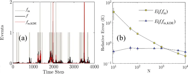
FIG. 3. (a) An example distribution f(x) with corresponding fm and fm,KDE distributions for
N = 100 and SN Rm = 0. (b) E(f, fm) and E(f, fm,KDE) as functions of N, showing that KDE
techniques provide better estimates off for smallN, with a relative error nearly independent ofN.
Ten sets of samples were obtained from f for each data point. The mean and standard deviation
of E for the 10 sets are shown for each as the data marker and error bars, respectively.
such cases the ratio fnoise(xi)/fm,KDE(xi) can still be very small, leading to Pnoise(xi) ≈ 0 and the measured event not being removed, as desired. The most sensitive SNR regime
for noise removal will therefore be SN Rm →0, and for such a regime it is imperative that fm,KDE(xi)≈f(xi).
The distribution f(x) from Figure 2 and its corresponding fm,KDE distribution with SN Rm = 0 are shown in Figure 3. fm,KDE clearly provides a better estimation of f(x) than the samples forming fm(x). To quantify this improvement, E(f, fm) andE(f, fm,KDE) are computed for various N values as shown in Figure 3b. For large N, the KDE distribu-tions have a slightly higher relative error than fm, but for small N they are more accurate by two orders of magnitude.
In the case of noise modeling for TOF-MS, KDE techniques can be applied for any
accu-mulation, such as time history, TOF, or incident particle direction datasets. For the incident
particle direction datasets, the bandwidth can apply to a two-dimensional Gaussian kernel.
In general, KDE techniques can be applied to higher-dimensioned datasets22, with each
di-mension permitted its own characteristic bandwidth. The visualization of such techniques
becomes difficult, and in the case of TOF-MS, the determination of appropriate bandwidths
may become intractable. For this reason, KDE techniques for TOF-MS may be practically
[image:11.612.138.464.79.208.2]with a Monte Carlo event processing algorithm should result in the misidentification of less
than 25% of all events, only a modest increase in overall error when compared with using a
known f(x) instead of fm,KDE(x) (determined as <20% in Appendix A) .
III. FORWARD MODELING OF INSTRUMENT NOISE
A good estimate of fnoise(x) is vital for an accurate noise removal. Furthermore, even in the absence of a suitable approximation for f(x), fnoise(x) will provide a direction esti-mation of instrument SNR. The complete fnoise(x) distribution should have contributions from any and all noise sources in an instrument. Here, the MESSENGER/FIPS sensor is
used as a baseline, and both background and active noise sources will be discussed and
modeled appropriately to demonstrate how to generate fnoise(x) from a set of accumulated observations.
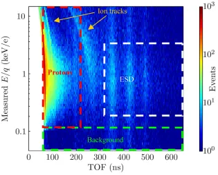
An unfiltered 50-day accumulation from the day-of-year (DOY) range 100–149 in 2011
of all MESSENGER/FIPS-measured events is shown in Figure 4. The E/q of each event is plotted as a function of TOF, with curved tracks corresponding to real events that are
superimposed onto various noise sources. This time period of data will serve as the
cali-bration dataset that will be used to characterize the behavior of fnoise. Data from the E/q steps marked as ”Background” will be used to characterize the background noise rates and
distributions. The distributions of events from the E/q−T OF steps marked as ”Protons” will be used to model the contamination of the H+ mass peak into the peaks for species
of higher mass per charge (m/q) ratios. Finally, the events within the E/q−T OF steps marked as ”ESD” will provide the rates of events triggered by increased electron-stimulated
desorption (ESD) of material from the start MCP at times of high incident particle flux.
The distribution of each of the active noise sources will be extrapolated to theT OF region 200–300ns, a range over which neither source appears to be dominant.
A. Passive noise sources
FIG. 4. (a) E/q−T OF spectrogram of 50 days (day of year 100-149 in 2011) of orbital
MES-SENGER/FIPS heavy-ion (m/q >1 amu/e) measurements. Curved tracks correspond to incident
ions. Boxes marking theE/q−T OF steps corresponding to background events, proton tail events,
and induced electron-stimulated desorption events are indicated as ”Background”, ” Protons”, and
”ESD”, respectively, and will be used to characterize each noise source.
background electron sources have been identified, as described by Gilbert et al.1: emission
from high-voltage wire harps, and a localized field emission source near the edge of the
MCP active area. A complete noise model must include distributions corresponding to each
source.
The E/qsteps marked as ”Background” in Figure 4 are the lowest instrument energy per charge steps over which few numbers of real ion events are expected, particularly outside
of Mercury’s magnetosphere. To further avoid possible contamination from any actual low
energy per charge events, only time steps where the ratio between the start MCP rate and
valid event rate was greater than 10 are used, as real incident events will have ratios of∼2 due
to the efficiencies of ion detectors. Due to frequent drifts in instrument operating conditions,
most notably ambient temperature, the background rate calculations were performed from
[image:13.612.145.460.81.335.2]signal on the start MCP (F SRbg); the ”rear” rate, i.e., the background signal on the stop
MCP (RSRbg); the background proton event rate, i.e., background events with low T OF, (P Ebg); and the valid event, i.e., the double-coincidence, background rate (V Ebg). These
rates (in units of s−1) are used in various stages of the instrument noise forward model. The accumulation time in seconds for each time step, ∆(t), is readily calculable and can
change with the operating mode of the instrument. The background T OF and MCPx−y spectra are obtained using the full 50-day accumulated dataset, since they are not expected
to change quickly with time.
The total background distribution must be separated into its harp emission and other
field emission subcomponents, denoted with subscripts ”he” and ”fe” respectively. A simple
separation isolates events corresponding to the ”hotspot” pixels (Gilbert et al.1) in the
background MCP x−y distribution as the generalized field emission source and attributes the rest to wire harp emission of electrons. Following Gilbert et al.1, theT OF distribution of the harp emission source corresponds to the flight times of desorbed ions from the surface
of the start MCP to the top of the TOF chamber. TheT OF of the field emission source also includes a set of peaks at a constant fraction of the flight times of the harp emission source,
indicating that desorbed species are striking the sides of the TOF chamber instead of the
top. These accumulated distributions are smoothed to reduce statistical noise. The resulting
distributions of MCPx−y and smoothed-T OF for each source are shown in Figures 5 and 6, respectively.
The T OF background noise distributions fnoise,fe(t, T OF, xMCP, yMCP) and
fnoise,he(t, T OF, xMCP, yMCP) can be written for a given accumulation of time following equa-tions (11) and (12),
fnoise,fe(t, T OF, xMCP, yMCP) =gfe·V Ebg ·fˆfe(T OF)·fˆfe(xMCP, yMCP)·∆(t), (11)
and
fnoise,he(t, T OF, xMCP, yMCP) =ghe·V Ebg ·fˆhe(T OF)·fˆhe(xMCP, yMCP)·∆(t). (12)
FIG. 5. Normalized MCP x−y distribution of background ESD events in MESSENGER/FIPS
triggered by (a) harp emission electrons ( ˆfhe(xMCP, yMCP)) and (b) field emission electrons
( ˆffe(xMCP, yMCP)). The red circle indicates the boundaries of the MCP active area. The field
emission electrons are concentrated in a beam forming a set of ”hotspot” pixels near the edge of
the active area whereas the harp emission electrons strike almost uniformly over the surface of the
MCP.
FIG. 6. NormalizedT OF distribution for background ESD events in MESSENGER/FIPS triggered
by (a) harp electrons ( ˆfhe(T OF)) and (b) field emission electrons ( ˆffe(T OF)). The harp emission
T OF distribution corresponds to the flight times of desorbed species from the surface of the start
MCP to the top of the TOF chamber. The field emission events include a contribution from
desorbed ions that strike the side of the TOF chamber, leading to flight times at a constant
[image:15.612.140.460.441.566.2]B. Active noise sources
Active sources create noise as a function of incident particles or photons. Any external
stimulus capable of generating signals from the start and stop detectors is considered an
active source. The sources considered here will be ion energy straggling and induced ESD, as
discussed in detail by Gilbert et al.1. Accidental coincidences due to high flux or penetrating
radiation will not be modeled due to the extremely low SNR of measurements during those
time periods.
1. Ion energy straggling
Particles passing through a thin carbon foil lose some of their kinetic energy, a
phe-nomenon called ”energy straggling”24. The resulting distribution features a high T OF peak tail for each species. For a TOF-MS, H+ will always have the smallest T OF, as it has the smallest possible m/q of 1 amu/e. The tail for H+, therefore, has the potential to con-taminate the T OF channels corresponding to all other ion species, as shown in Figure 4. Furthermore, for MESSENGER/FIPS, the most easily measured ion is H+, which is present
in both the solar wind and Mercury’s magnetospheric environments and is typically orders
of magnitude more abundant than other species25. The rates of heavier ion events can be
comparable to the magnitude of the proton peak tail, making it difficult to distinguish
be-tween the two sets of particles. Events in the E/q− T OF steps in Figure 4 labeled as ”Protons” are assumed to be dominated by the proton peak tail.
Although it is possible to obtain an overall good fit to energy-straggled T OFs using a kappa distribution24, for heavy ion species small errors in the fit can create relatively large
er-rors infnoise. Therefore, rather than use a functional fit for the entire proton peak shape, the accumulation of data from Figure 4 is smoothed and used as the noise distribution directly,
analogous to the formation of the background noise distributions. The average proton peak
shape is expected to change with time, as changes in ambient temperature may affect the
energy straggling process through the carbon foil, and the thickness of the carbon foil may
not be spatially uniform, leading to different peak shapes for time periods where, on average,
particles enter the instrument aperture from different directions. For MESSENGER/FIPS,
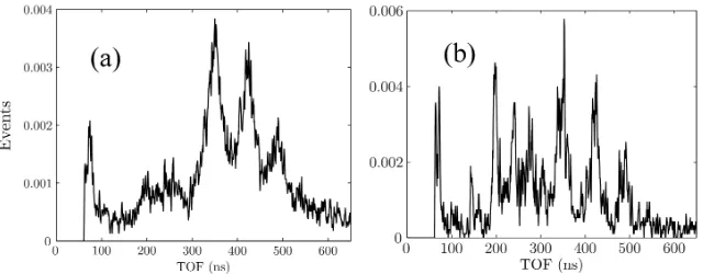
FIG. 7. T OF distribution of proton tail events fromE/q = 1.5 keV/e for DOY 100–209 in 2011,
normalized by the proton event rate. T OFs corresponding to solar wind ion tracks for He2+, He+,
and hOCi, the averaged solar wind heavy ions3, are indicated. The black solid curve is the set of
normalized raw measurements . The red dashed curve represents a smoothed curve that has been
interpolated through ion track T OFs and extrapolated to higher T OFs with a power law.
statistical significance and capturing this time variation.
The expected background spectum calculated in Section III A is subtracted from this
accumulation, andT OF channels corresponding to actual ion tracks are excluded. The data are linearly interpolated through these data gaps and extrapolated to higher T OF channels with a power-law fit, consistent with a kappa T OF peak shape. An example T OF spectra for a 10-day accumulation at E/q = 1.5 keV/e is shown in Figure 7, with a corresponding noise curve fit that interpolates through ion track locations and extrapolates to higherT OF values.
The amplitude of the H+ tail should scale with the total number of measured proton
events (PE) measured at lower T OFs, i.e., near the peak of the H+ T OF distribution. The accumulated data in each energy step is therefore normalized by the total corresponding
for energy steps in which the proton event rate is comparable to the background rate.
However, since the expected noise from proton events in these steps will be low, this error is
manageable. The MCP x−ydistribution of this noise will be that of the incident protons, ˆ
finc,H+(E/q), which can be obtained by accumulating events close to the proton peak at each energy step. The expected fnoise therefore becomes:
fnoise,H+(t, T OF, E/q, xMCP, yMCP) = (P E(t, E/q)−P Ebg)
×fˆnoise,H+(T OF, E/q)
×fˆinc,H+(xMCP, yMCP)
×∆(t). (13)
2. Induced ESD
In addition to electrons from field emission or harp emission sources, secondary electrons
from incident particles can desorb ions from instrument surfaces, resulting in valid T OF events. For MESSENGER/FIPS, a number of ion species are desorbed from the start MCP
and follow trajectories that lead to correlated stop signals. This effect occurs with some
probability relative to an incident particle being detected. Therefore, the total number of
these events should be proportional to the number of non-background start signals detected
in a particular E/q step. Also, desorption rates will depend not only on the number of incident particles but on where those particles enter the instrument.
Given, as in Section III A, that a uniform distribution of harp electrons strikes the MCP,
the harp electron event distribution is proportional to the number of valid events per start
signal in each MCP ”pixel”. Not every start signal will have a corresponding stop signal, so
the ratio of the valid event rate to the start rate will always be less than one. In addition, the
incident particle distribution ( ˆfinc) should correspond to the distribution of start signals on the MCP. Multiplying ˆfinc(xMCP, yMCP) by the background harp electron event distribution
ˆ
fhe,bg(xMCP, yMCP) should therefore give an estimation of the MCP spatial distribution of induced ESD events.
on average tend to hit closer to the center of the MCP active area than the background
events. Ions desorbed from these locations have a larger distance to travel due to the curved
top of the TOF chamber. This effect is observed as a small shift inT OF (T OFo) of the harp electronT OF distribution. For MESSENGER/FIPS,T OFo can be computed for each daily accumulation of data through the calculation of the change in the first moment of the largest
T OF peak (325–375ns) from the expected background distribution, following equation (14),
T OFo = X ESD
T OF ·(fm−fhe,bg)
X ESD
(fm−fhe,bg)
−
X ESD
T OF ·fhe,bg
X ESD
fhe,bg
, (14) where X ESD ≡ 375ns X TOF=325ns X (E/q)ESD
X t
X (xMCP,yMCP)
. (15)
The distribution of ESD-induced noise with respect toE/q step and MCPx−ycan then be written as,
fnoise,ESD(t, xMCP, yMCP, E/q) =c·(F SR(t, E/q)−F SRbg)
×fhe(t, xMCP, yMCP)ˆ
×fˆinc(t, xMCP, yMCP, E/q)
×fˆhe,bg(T OF −T OFo)
×∆(t), (16)
where c is a constant.
The constant c can be found from a daily accumulation of data such that,
X ESD
(fm−fhe,bg) = X ESD
fnoise,ESD. (17)
With a full TOF spectrum of noise known, the ESD spectrum readily applies to the
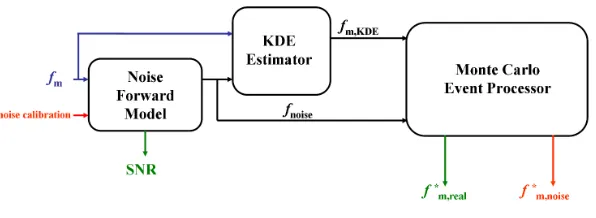
FIG. 8. Block diagram describing noise modeling and event processing for MESSENGER/FIPS.
Measured data as well as noise calibration factors are input into a noise forward model that produces
fnoiseand consequently, estimates of dataset SNR. The measured datafmalong withfnoiseis input
to a KDE estimator that providesfm,KDE, a distribution suitable for use in a Monte Carlo processor
that separates fminto fm∗,real and fm∗,noise.
IV. NOISE PROCESSING FOR MESSENGER/FIPS
As illustrated in Figure 8, with all noise sources well characterized,fnoisecan be accurately determined for a given set of measured data fm, resulting in a direct estimation of SNR for any size dataset. A KDE estimator, given fnoise and fm as inputs, can produce fm,KDE, an approximation to the underlying distribution function (f) that can be analyzed using a
Monte Carlo event-processing algorithm, and the measured distribution of real events,fm∗,real, can be recovered. This model is applied here to in-flight data from MESSENGER/FIPS.
A. Noise forward modeling
To model the various sources of noise, the relevant noise distributions from Section III
must be added together for each time step. It is important to note that the spatial
distribu-tion of incident particles is required in both the models of proton peak tail noise and induced
ESD events for MESSENGER/FIPS. When the SNR in each E/q step is low, an iterative noise removal/modeling process may be required to obtain the proper incident spatial
distri-bution. However, in the case of MESSENGER/FIPS, the number of expected noise events
will be small for a single time step, i.e., fm,noise(t) fm,real(t). E/q steps that contribute substantially to active noise sources will have large numbers of incident particles that should
is used for an approximation to the spatial distribution of incident particles. The error in
this approximation will be large for small numbers of incident particles, but since active
noise sources scale with the measured start rate, the contribution from these low count-rate
steps to the total accumulated active noise should be negligible.
Due to the number of data dimensions and their corresponding interdependencies, a
complete five-dimensional fnoise(t, E/q, T OF, xMCP, yMCP) distribution may be difficult to manage and store. Furthermore, as discussed in Section II B, noise removal using KDE
techniques is challenging for higher-dimensional datasets. Therefore, instead of producing
the complete distribution of noise, several noise data products can be produced that represent
accumulations along one or more of the dimensions. Such summation seemingly removes
vital information for reconstructing an accurate fm,real. However, as will be discussed in Section IV B 1, with proper choice of accumulations, a reasonable fm,real can be recovered. For MESSENGER/FIPS, the MCP x−y distribution is measured with the least precision. Furthermore, the majority of the noise sources are either widely spread over the MCP active
area or have a similar positional dependence as the incident particles. Therefore, ignoring
the MCP x−y dependence is expected to improve statistical significance of accumulations with minimal impact on the accuracy of modeled distributions.
Two accumulations are calculated here as an example. The first, fnoise, is a E/q−T OF spectrogram for a particular time period. Such an accumulation, although not as useful from
the perspective of scientific analysis, provides a good evaluation of noise forward-modeling
performance. The second, fnoise, is an energy-dependent time series for a given ion that accumulates over MCP x−y and several T OF values, and that series will be the baseline for all FIPS heavy ion science analysis.
An accumulatedE/q−T OF distribution (9a) with corresponding forward modeled noise (9b) for 10 days (DOYr 100–109, 2011) in shown in Figure 9. Ion tracks for He2+, He+, Na+,
and Ca+ are marked. For clarity, not all ion tracks present in the data have been included.
The two distributions vary only at the locations of ion tracks, where the noise distribution
underestimates the total number of events, as expected. There are good matches with the
FIG. 9. (a) 10 day (DOY 100–109, 2011) E/q−T OF accumulation of events measured by
MES-SENGER/FIPS. Tracks corresponding to heavy ions He2+, He+, Na+, and Ca+ are highlighted.
(b) Forward modeled E/q−T OF noise distribution for the same time period. There is an
ex-cellent match between the measured data and generated fnoise distribution, with the only major
discrepancies occurring at the locations of known ion tracks, at which actual events are expected
to be present.
data.
B. Noise removal
Once fnoise is generated, the set of processed events can be split into sets of recovered real and noise-based events. Although it is not possible to calculate the accuracy of this
separation for measured datasets, the expected properties of recovered events, both real and
noise, can be used to gain confidence in the removal process. On-orbit MESSENGER/FIPS
data (DOY 100–109, 2011) have been analyzed using daily accumulations of He2+, He+,
Na+, and Ca+ at eachE/q step, yielding a series of one-dimensional time series suitable for processing with the algorithm described in Section II A 2.
Each time series is further split into two parts: ”active” and ”quiet”, with active times
defined as periods when the proton rate goes above 15 events per E/q step (i.e., inside
Mercury’s magnetosheath or during FIPS solar wind observations), and quiet times
(typi-cally inside Mercury’s magnetosphere) defined as when the proton rate has remains below
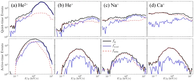
[image:22.612.140.471.84.232.2]FIG. 10. Total measured (fm), modeled noise (fnoise), and recovered ion events (fm∗,real) as a
function of E/qfor a 10 day (DOY 100–109, 2011) accumulation of MESSENGER/FIPS on-orbit
data for quiet and active periods for (a) He2+, (b) He+, (c) Na+, and (d) Ca+. The noise processing
algorithm accurately recovers ion events, resulting in a substantial increase in measurement
signal-to-noise ratios, especially for E/qsteps corresponding to a high incident proton flux.
depending on operating mode). The active time periods will be dominated by active noise
sources such as H+ energy straggling and induced ESD, which have larger uncertainty in
the forward modeled fnoise. If the noise for a particular step is overestimated, real events that occur during quiet times would be thrown out. By splitting up the time series, a more
sensitive recovery of events is expected.
The total number of events from both active and quiet time periods for each ion as a
function of E/q is shown in Figure 10, along with corresponding recovered real events and predictedfnoise. For all ions, the large peak near E/q= 1 keV/e is effectively removed, since it corresponds to the proton peak tail/ESD events. From Figure 9, where there are clear ion
tracks at higher energies in the absence of modeled noise, almost no events are removed.
Statistics will also play a role in the recovery, as the counting error (√N) for low SNR datasets results in some uncertainty on the number of events that should be eliminated.
Consequently, the threshold ratio of the recovered signal to counting error ratio, S/√N, may be required to give confidence in the recovery even in the presence of errors in the noise
forward model. For example, in the analysis of Gershman et al.3, Zurbuchen et al.2, and
[image:23.612.138.469.71.210.2]ensure that times of increased solar wind proton flux into the instrument did not lead to an
erroneously high measurement of He+ events.
1. Recovery of individual ion events
The output of the noise processing algorithm is a one-dimensional time history of ion
events as a function of E/q. However, to enable the most flexibility in scientific analysis of measured instrument data, a list of real individual events in the full five dimensions is
desired. Surprisingly, the low measurement statistics are actually advantageous for this
recovery. The processed dataset will have at most a few measured events (often only one)
per time step. For this case, there is very little ambiguity on which event per step should be
identified as noise. However, in cases with multiple events per time step, a simple criterion
is used in which the proper number of events with the highest predicted MCP x−y noise for that particular step are removed. Such a recovery will result in increased error, but this
ambiguity will not be common for low statistics, and in fact datasets with large numbers of
events will most likely not require such a recovery. Furthermore, the effects of any errors
introduced by incorrect assignment of events are expected to be small, especially since most
noise events have MCP distributions similar to those of actual events.
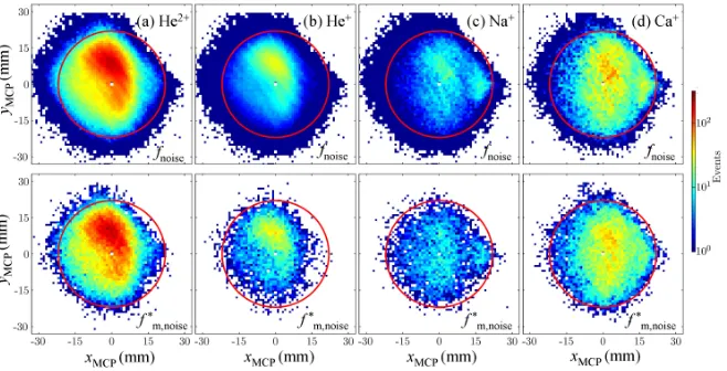
As an example, Figure 11 shows the total modeled MCP x−y noise distribution for He2+, He+, Na+, and Ca+, and the corresponding MCPx−ydistributions of the recovered noise events, fm∗,noise. The overall recovery errors are expected to be less than 25% as predicted by the example distributions from Appendix B. The removed noise events exhibit a
similar distribution to the predicted noise in terms of both spatial distributions and intensity.
Therefore, despite the fact that the MCP x −y distribution was not considered during the removal process, a reasonable five-dimensional event distribution recovery has been
accomplished.
V. CONCLUSIONS
We have developed a mathematical framework for the characterization, forward
mod-eling, and post-processing of noise events in spaceborne time-of-flight mass spectrometers.
FIG. 11. Total recovered and modeled noise MCPx−y distributions for DOY 100–209, 2011 for
(a) He2+, (b) He+, (c) Na+, and (d) Ca+ions. The recovered noise MCPx−ydistributions are the
set of individual events (with full five-dimensional information) that have been processed with the
Monte Carlo noise removal algorithm. Although the MCPx−ydependence was originally ignored
in the event processing, the recovered distribution,fm∗,noise, still matches the predicted noise,fnoise,
implying a quality removal.
was constructed that provided estimations of the ratio of signal to noise in all data
dimen-sions. Kernel density estimation techniques were used to take measured instrument data
and recover their underlying distribution functions suitable for use with a Monte Carlo
event-processing algorithm. With an accurate noise model, measured events were separated
into real and noise-based events, with an expected overall misidentification of events
ex-pected to be less than 25%, even for datasets with low SNR or poor counting statistics.
This removal was done after accumulating over incident particle directions that were later
recovered, enabling maximum versatility in possible scientific analysis.
Although applied to MESSENGER/FIPS as an example, the techniques described here
are applicable to any such TOF-MS or even other sensors that measure discrete events.
An in-depth characterization of noise not only results in an improved understanding of
idiosyncrasies of a particular spaceflight instrument, but can also make any changes in
sensor response or newly measured scientific phenomena more easily identifiable. These
techniques provide a way to improve the SNR of instruments for which settings may not
be sufficiently adjustable in flight, a method to mitigate unexpected instrument behavior
plagued with low SNR can be revisited and potentially reanalyzed, producing new scientific
results from all-but-forgotten instruments.
Appendix A: Event processing errors
Before being applied to in-flight data, the performance of the removal process must be
evaluated with synthetic datasets. A direct calculation of the change in SNR after processing
data is not necessarily an adequate metric in determining the accuracy of the noise removal.
In fact, the results of such a computation may be misleading as, in addition to removing
noise-based events, an algorithm may remove some real events, biasing measurements of
SNR. Therefore, the relative loss of signal, |∆S/S|, and relative reduction in noise, |∆η/η|,
should be analyzed individually. Note that with the presented technique, the total number of
recovered real events will be set by the total amount of modeled noise, so errors in processing
will likely be a misclassification of noise and real events rather than removal of the incorrect
number of events. Therefore, it is expected that |S| ≈η− |∆η|.
Steps that contribute to data loss are those for which the total remaining signal (fm∗,real) is less than that of the distribution of true real events (fm,real). Accumulating these differences
and dividing by the total number of real events yields the fraction of events lost due to the
removal process,|∆S/S|, as shown in equation (A1),
∆S S =X i
fm,real(xi)−fm∗,real(xi) X
j
fm,real(xj)
, fm,real(xi)≥fm∗,real(xi)
0, fm,real(xi)< fm∗,real(xi)
. (A1)
On the contrary, steps that overestimate the real signal, i.e., fm∗,real > fm,real, can be used according to equation (A2) to calculate the fraction of the noise removed, |∆η/η|,
∆η η
= 1−X
i
fm∗,real(xi)−fm,real(xi) X
j
fm,noise(xj)
, fm∗,real(xi)≥fm,real(xi)
0, fm∗,real(xi)< fm,real(xi)
. (A2)
from data and can be used in the analysis only of synthetic datasets. Ideally, |∆S/S| → 0
and |∆η/η| →1, i.e., all of the noise is removed without eliminating any of the true signal.
The overall misidentification of events (|∆f /f|) can be calculated by adding the number
of removed signal events (∆S) to the number of remaining noise events, (η− ∆η), and
normalizing by the total number of events, N,
∆f f
= S+ (η−∆η)
N . (A3)
From the known relationships between S,η, and SN Rm,
S =N · SN Rm
1 +SN Rm and
η=N · 1
1 +SN Rm, (A4)
(A5)
and combining these relations with equations (A1) and (A2), equation (A3) can be written
as, ∆f f = 1
1 +SN Rm 1− ∆η η
+ SN Rm 1 +SN Rm
∆S S . (A6)
As expected, for the ideal recovery in which |∆S/S| →0 and|∆η/η| →1, the
misclassi-fication of events |∆f /f| →0.
As discussed in Section II A 2, Pnoise is used instead of Pm,noise as part of an iterative Monte Carlo event processing technique. The error introduced by this approximation can
be quantified through Monte Carlo processing of two synthetic datasets. Two test cases are
examined: (1) real events uniformly distributed in time, and (2) real events all occurring at
a single time step. Noise sampled from the distribution shown in Figure 2 is superimposed
on each signal.
In the case of a perfectly localized signal, Pnoise = Pm,noise. Therefore, even for small N, a Monte Carlo processing technique will separate fm,real and fm,noise with almost 100% accuracy, with |∆S/S| ≈ 0 and |∆η/η| ≈ 1. For a uniformly distributed signal, however,
FIG. 12. (a) |∆S/S|, (b) |∆η/η|, and (c) |∆f /f| as functions of SNR of a uniformly distributed
real event signal for various numbers of noise-based events η. An idealized Monte Carlo event
processing algorithm was used with Pnoise computed using the noise distribution from Figure 2.
Each data point represents the average of 10 independent removals of the same dataset, and the
error bars indicate the standard deviation. The overall misidentification of events, |∆f /f|, is less
than 20% for all SNR.
and|∆f /f|may be computed for a varying number of noise-based eventsη = 10, 100, 1000, and 10,000 and are shown in Figure 12.
Both fewer real and noise events are removed with increasing SNR, with approximately
a 20% removal of real events and 80% removal of noise events at SNR ≈ 1 in Figures 12a
and 12b. The overall event identification error, |∆f /f|, in Figure 12c, however, is less than
20% for all SNR, peaking near SNR ≈ 1. Event misidentification is a consequence of using
the large N limit noise probability Pnoise instead of Pm,noise. These errors will be greatest for non-localized event distributions. As expected, improved results are obtained for large
N, where Pm,noise → Pnoise. However, despite these misidentifications, it is important to remember that the algorithm will necessarily remove the correct amount of noise, i.e., the
total amount of recovered signal will be accurate to within the errors of fnoise.
Appendix B: Event processing errors from KDE
With appropriately defined metrics |∆S/S|,|∆η/η|, and |∆f /f|, the performance of a
KDE-implemented noise removal algorithm can be analyzed using synthetic data as a
func-tion of the total number of events and dataset SNR. The two test cases used in Appendix A
[image:28.612.138.474.72.161.2]FIG. 13. (a), (b), (c) are the same as Figure 3 but withfm,KDEinstead of a knownf for a uniform
distribution of real events. (d),(e),(f) are the same as parts (a),(b), and (c) but for a localized
event source at time step t = 2800. With KDE techniques, the overall misidentification error is
expected to be less than 25%.
For the uniform real event distribution, the |∆S/S|,|∆η/η|, and |∆f /f| values here are
similar to the ideal Monte Carlo process results from Figure 12, with slightly more real events
being misidentified at SNR = 1 (∼25%) and slightly less noise events removed at higher SNR
values (∼20%). The localized events also show some increased error when compared with
the idealized case. As expected, an increased number of events N leads to more accurate removal. The KDE technique therefore appears to provide suitable estimates of f(x), such that the end result of the Monte Carlo processing algorithm is similar to that of the ideal
cases in all SNR regimes. From these tests, one can expect that for an accurate fnoise, the total number of expected noise events will be removed with less than 25% of the total events
(noise and real) being misidentified for both localized and more uniform distributions of real
events.
ACKNOWLEDGMENTS
The MESSENGER project is supported by the NASA Discovery Program under contracts
NAS5-97271 to The Johns Hopkins University Applied Physics Laboratory and
NASW-00002 to the Carnegie Institution of Washington. This work was also supported by the
[image:29.612.137.472.75.243.2]like to thank Sean C. Solomon for his assistance with the preparation of this manuscript.
REFERENCES
1J. A. Gilbert, D. J. Gershman, G. Gloeckler, R. A. Lundgren, T. H. Zurbuchen, T. M.
Orlando, J. McLain, R. von Steiger, Characterization of background noise in space-based
time-of-flight sensors, Rev. Sci. Instrum., (2013), in revision.
2T. H. Zurbuchen et al., Science, 333, 1862–1865, (2011), doi:10.1126/science.1211302.
3D. J. Gershman, T. H. Zurbuchen, L. A. Fisk, J. A. Gilbert, J. M. Raines, B. J. Anderson,
C. W. Smith, H. Korth, S. C. Solomon, J. Geophys. Res., 117, A00M02, 14 pp, (2012),
doi:10.1029/2012JA017829.
4D. J. Gershman, G. Gloeckler, J. A. Gilbert, J. M. Raines, L. A. Fisk, S. C. Solomon,
E. C. Stone, T. H. Zurbuchen, J. Geophys. Res. Space Physics, 118, 1389–1402, (2013),
doi:10.1002/jgra.5022.
5J. M. Raines et al., J. Geophys. Res. Space Physics, 118, 1604–1619, (2012),
doi:10.1029/2012JA018073.
6T. H. Zurbuchen, G. Gloeckler, J. C. Cain, S. E. Lasley, W. Shanks, in Conference on
Missions to the Sun II, ed. by C. M. Korendyke, Proceedings of the Society of
Photo-Optical Instrumentation Engineers, Bellingham, Wash., vol. 3442, 1998, pp. 217–224.
7G. B. Andrews, et. al., Space Sci. Rev., 131, 523–556 (2007)
doi:10.1007/s11214-007-9272-5.
8S. C. Solomon et al., Planet Space Sci., 49, 1445–1465, (2001),
doi:10.1016/S0032-0633(01)00085-X.
9V. P. Tuzlukov, Signal Processing Noise, 1st ed. (CRC Press, Boca Raton, FL, 2002), 688
pp.
10H. Kuo, White Noise Distribution Theory, 1st ed. (CRC Press, Boca Raton, FL, 1996),
400 pp.
11S. V. Vaseghi, Advanced Digital Signal Processing and Noise Reduction, 4th ed. (John
Wiley, Hoboken, NJ, 2009), 544 pp.
12R. C. Gonz´alez and R. E. Woods, Digital Image Processing, 3rd ed. (Prentice Hall, Upper
Saddle River, NJ, 2007), 976 pp.
Analysis and Applications, 1st ed. (Academic Press, Waltham, MA, 2010), 856 pp.
14A. Smirnov, Processing of Multidimensional Signals, 1st ed. (Springer-Verlag, Berlin,
1999), 284 pp.
15G. M. Davis, Noise Reduction in Speech Applications, 1st ed. (CRC Press, Boca Raton,
FL, 2002), 432 pp.
16M. H. Kalos and P. A. Whitlock, Monte Carlo Methods, 2nd ed. (John Wiley, Hoboken,
NJ, 2008), 215 pp.
17K. Binder and D. W. Heerman, Monte Carlo Simulation in Statistical Physics: An
Intro-duction, 5th ed. (Springer, New York, 2010), 214 pp.
18B. F. J. Manly, Randomization, Bootstrap and Monte Carlo Methods in Biology, 3rd ed.
(CRC Press, Boca Raton, FL, 2006), 480 pp.
19P. Glasserman, Monte Carlo Methods in Financial Engineering, 1st ed. (Springer, New
York, 2003), 616 pp.
20D. T. Young, et al., Space Sci. Rev., 114, 1–112 (2004), doi:10.1007/s11214-004-1406-4.
21D. W. Scott, Multivariate Density Estimation: Theory, Practice, and Visualization, 1st
ed. (John Wiley, Hoboken, NJ, 1992), 376 pp.
22B. W. Silverman, Density Estimation for Statistics and Data Analysis, 1st ed. (CRC Press,
Boca Raton, FL, 1986), 176 pp.
23R. L. Graham, D. E. Knuth, O. Patashnik, Concrete Mathematics: a Foundation for
Computer Science, 2nd ed. (Addison-Wesley, Boston, MA, 1994), 657 pp.
24F. Allegrini, D. J. McComas, D. T. Young, J. Berthelier, J. Covinhes, J. Illiano, J.
Riou, H. O. Funsten, R. W. Harper, Rev. Sci. Instrum., 77, 044501, 7pp, (2006)
doi:10.1063/1.2185490.