E stim a tio n o f fractional co-in tegration
w ith unknow n in tegration orders
Thesis submitted for the degree of
UMI Num ber: U 1 8 8 0 6 2
All rights r e serv e d
INFORMATION TO ALL U S E R S
T h e quality o f this reproduction is d e p e n d e n t upon th e quality of th e c o p y su bm itted .
In th e unlikely e v e n t that th e author did not s e n d a c o m p le te m an u scrip t
and th ere are m issin g p a g e s , t h e s e will b e n oted . A lso , if m aterial had to b e rem oved , a n ote will ind icate th e d eletio n .
D issertation Publishing
UMI U 1 8 8 0 6 2
P u b lish ed by P ro Q u est LLC 2 0 1 4 . C opyright in th e D isserta tion held by th e Author.
Microform Edition © P ro Q u est LLC.
All rights r e se r v e d . T his work is protected a g a in s t
u nau th orized cop y in g under Title 17, United S ta te s C o d e .
P ro Q u est LLC
7 8 9 E a st E ise n h o w e r Parkw ay
OF FOJTICAL
AND
F
A b stra ct
C on ten ts
1 In tro d u ctio n 8
1.1 The concept of in te g ra tio n ... 9
1.2 The concept of c o -in te g ra tio n ... 13
1.3 Estimation of co-integrating r e la tio n s ... 16
1.3.1 First stage p r o c e d u r e s ... 17
1.3.2 Second stage p ro c e d u re s ...22
1.4 Empirical evidence of fractional c o -in te g ra tio n ...32
1.5 Description of the t h e s i s ... 34
2 P aram etric estim a tio n o f stron g fractional co -in tegration 37 2.1 In tro d u c tio n ... 37
2.2 Estim ates of co-integrating p a r a m e te r s ...39
2.3 Conditions and main r e s u l t s ...42
2.4 Monte Carlo evidence...47
2.4.1 Performance for different combinations of o r d e r s ... 50
2.4.2 Standard situation: 7 = 0, 6 =1 ... 55
2.5 Empirical investigation: the purchasing power parity hypotheses . . . 56
2.6 Final c o m m e n ts... 59
2.7 Appendix 2 ...60
2.7.1 Appendix 2.A: Outline of proof of Theorem 2.1 ...60
2.7.2 Appendix 2.B: Proofs of p ro p o s itio n s ...63
2.7.3 Appendix 2.C: Technical l e m m a s ... 71
2.7.4 Appendix 2.D: Lemmas concerning th e aa w e ig h ts ... 74
3 P aram etric estim a tio n o f w eak fractional co-in tegration 99 3.1 In tro d u c tio n ...99
3.2 Estim ation of v ...101
3.3 Asymptotic theory w ith known 7, 8 ... 103
3.4 The case of unknown 7, 6 ... 105
3.5 Monte Carlo evidence... 108
3.6 Empirical e x a m p le s ... 112
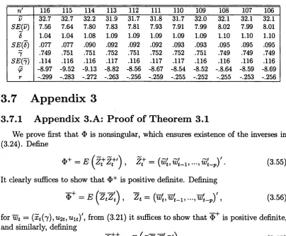
3.7 Appendix 3 ...116
3.7.1 Appendix 3.A: Proof of Theorem 3 . 1 ... 116
4 S em ip aram etric estim a tio n o f stro n g and w eak co-in tegration 137
4.1 In tro d u c tio n ...137
4.2 The “optimally” weighted class of e s t i m a t e s ... 138
4.3 The “zero-frequency” weighted class of estim ate s...145
4.4 Monte Carlo evidence... 147
4.4.1 Strong fractional c o -in te g ra tio n ...148
4.4.2 Weak fractional co -in teg ratio n ... 154
4.5 Appendix 4 ... 156
5 T estin g for th e eq uality o f orders o f in teg ra tio n 247 5.1 In tro d u c tio n ...247
5.2 Testing the equality of fractional difference p a r a m e t e r s ...248
5.3 Monte Carlo evidence...254
List of Tables
C hapter 2.2.1 2.2 2.3-2.6 2.7-2.10 2.11-2.14 2.15-2.16 2.17-2.20 2.21-2.24 2.25-2.28 2.29-2.30 2.31 2.32-2.35 2.36-2.39 2.40-2.41 2.42 2.43 2.44
C hapter 3.
3.1 3.2 3.3 3.4 3.5 3.6-3.12 3.13-3.14 3.15 3.16-3.22 3.23-3.24 3.25 3.26-3.32 3.33-3.34 3.35 3.36 3.37 3.38-3.39 3.40 3.41 3.42-3.43
P aram etric estim a tio n o f stron g fractional co-in tegration
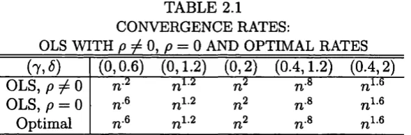
Convergence rates: OLS with p ^ 0, p = 0 and optimal rates P P P empirical example: estimates of v and Wald tests of v = 1 for models 1-7 computed from the last n ' = 113,..., 123 observations of U S/U K d ata
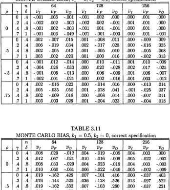
Monte Carlo bias, white noise Monte Carlo bias, AR(1) Monte Carlo bias, MA(1) Monte Carlo bias, ARM A (1,1)
Monte Carlo standard deviation, white noise Monte Carlo standard deviation, AR(1) Monte Carlo standard deviation, M A(1) Monte Carlo standard deviation, ARM A (1,1) Empirical sizes, white noise
Empirical sizes, AR(1) Empirical sizes, MA(1) Empirical sizes, ARM A (1,1) Monte Carlo bias for 6 — 1, 7 = 0
Monte Carlo standard deviation for 6 = 1, 7 = 0 Empirical sizes for 6 = 1, 7 = 0
P aram etric estim a tio n o f w eak fraction al co-in tegration
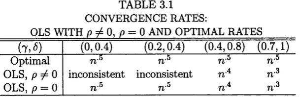
Convergence rates: OLS with p 0, p = 0 and optimal rates Consumption and Income: ut white noise
Consumption and Income: u u AR(1), u 2t white noise logM l and logGNP: ut white noise
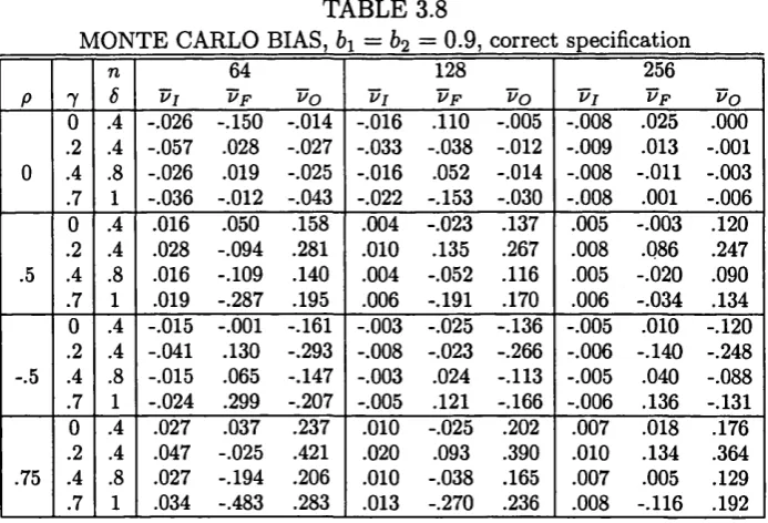
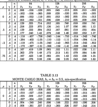
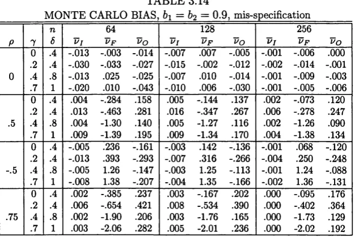
Stock Prices and Dividends: Ut white noise Monte Carlo bias, correct specification Monte Carlo bias, mis-specification Monte Carlo bias, over-specification
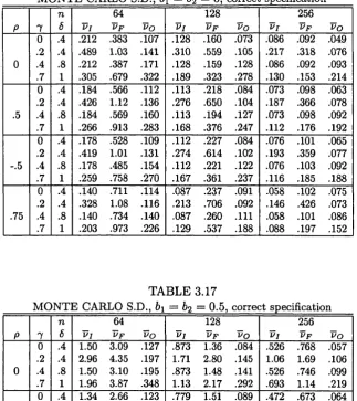
Monte Carlo standard deviation, correct specification Monte Carlo standard deviation, mis-specification Monte Carlo standard deviation, over-specification Empirical sizes, correct specification
Empirical sizes, mis-specification Empirical sizes, over-specification Monte Carlo bias of <5, p = 0.5
Monte Carlo standard deviation of <5, p = 0.5 Empirical sizes of Ws, p = 0.5
Monte Carlo bias of 7, p — 0.5
C hap ter 4. S em ip aram etric estim a tio n o f stro n g and w eak co -in teg ra tio n
4.1 Convergence rates: Band with p ^ 0, p = 0 and proposal 4.2-4.9 Monte Carlo bias, strong co-integration, white noise 4.10-4.25 Monte Carlo bias, strong co-integration, A R(1) 4.26-4.41 Monte Carlo bias, strong co-integration, MA(1)
4.42-4.49 Monte Carlo standard deviation, strong co-integration, white noise 4.50-4.65 Monte Carlo standard deviation, strong co-integration, AR(1) 4.66-4.81 Monte Carlo standard deviation, strong co-integration, M A(1) 4.82-4.89 Empirical sizes, strong co-integration, white noise
4.90-4.105 Empirical sizes, strong co-integration, AR(1) 4.106-4.121 Empirical sizes, strong co-integration, MA(1) 4.122-4.129 Monte Carlo bias, weak co-integration, white noise
4.130-4.137 Monte Carlo standard deviation, weak co-integration, white noise 4.138-4.145 Empirical sizes, weak co-integration, white noise
C hap ter 5. T estin g for th e eq u ality o f orders o f in tegration
0.5, param etric estimation 5.1 Empirical sizes of f2 (■) for p
5.2 Empirical sizes of t2 ( ) for p
5.3 Empirical sizes of t2 ( ) for p
5.4 Empirical sizes of t2 ( ) for p
5.5 Empirical sizes of t2 ( ) for p
5.6 Empirical sizes of t2 ( ) for p
5.7 Empirical sizes of t2 ( ) for p
Acknowledgments
First, I would like to thank especially Peter M. Robinson for his advice and careful supervision throughout the period I devoted to writing this thesis. I will be permanently indebted to him for his generous and invaluable help. I would also like to thank several other people who have helped me w ith this thesis at different stages. Thanks to Michele Arslan, Josu Arteche, Fabio Busetti, Xiaohong Chen, Luca Deidda, Jose E. Galdon, Luis Alberiko Gil-Alana, Luidas Giraitis, Javier Hidalgo, Fabrizio Iacone, Sue Kirkbride, Stepana Lazarova, Oliver Linton, Domenico Marinucci, Marcia Schafgans, Carlos Velasco and Jose Vidal. Thanks to Alan M. Taylor for providing the d ata I employed in C hapter 2, and very special thanks to Antonio Aznar, who originated my interest for econometrics. I would like to thank the Ramon Areces Foundation for its financial support, without which it would not have been possible to write this thesis. Financial assistance through ESRC G rant R000238212 and from the departm ent of economics a t the London School of Economics is also gratefully acknowledged.
C hapter 1
In trod u ction
Traditionally, co-integration analysis has developed almost exclusively in the con text of processes w ith non-fractional integration orders. Most popularly, observed series are assumed to have a single unit root, such th a t first differencing produces a weakly dependent, invertible stationary process, while co-integrating errors also sat isfy the latter description. This basic setting has been greatly extended, to observed series in which twice differencing is required to produce stationary weak depen dence, and to polynomial co-integration; polynomial time trends have also been introduced, and co-integration w ith respect to cyclic and seasonal frequencies has been examined. However, co-integration can exist among much more general non- stationary (and indeed stationary) observations, with stationary or non-stationary co-integrating errors, and it seems desirable to develop the topic in a broader con text, nesting the integer-order cases in a more general class, allowing integration orders to be real-valued. Undoubtedly, dealing w ith fractional processes could entail some difficulties, bu t in recent times, knowledge of their statistical properties has advanced considerably, so th a t issues like their role in co-integration analysis can be explored. In fact, fractional co-integration has become a relatively popular issue in the last decade among both theoretical and empirical econometricians, and this thesis mainly concentrates on one of the most relevant issues in this field, th a t is the estimation of a relation of fractional co-integration.
Before describing our aim in detail, we need to place this work in the right perspective. This Introduction has been w ritten with this idea in mind, stressing the connection between the wider framework th a t fractional co-integration allows and the traditional prescription of unit roots and standard co-integration.
1.1
T h e con cep t o f in tegration
Following Engle and Granger’s (1987) seminal work, a scalar series t G Z, Z = { t : t = 0, ± 1 ,...} , is integrated of order d, denoted traditionally ~ I (d) (see Definitions 1.2 and 1.3 below), if it has no deterministic component and could be represented as a stationary, invertible autoregressive-moving average (ARMA) after differencing it d times. Usually, the param eter d has been assumed to be 0, 1 or 2, the original series being modelled as I (0) processes without, or under first or twice differencing respectively. Undoubtedly, the key aspect of th a t definition is the concept of I (0) process, which in popular term s has been referred to as “short memory” , “weakly dependent” , “short-range dependent” or, in our view the most appropriate description, “weakly autocorrelated” process. The I (0) concept has taken different, although relatively closely related, shapes in the literature. W ith out the aim of being very exhaustive in an otherwise quite extensive field, we will comment on different ideas related to this issue.
Engle and Granger (1987) completed their above definition w ith some character istics th a t they attributed to I (0) processes. In particular, among other features, they stated th a t the spectral density of a covariance stationary 1(0) process / c (A), given by
1 00
(i-i)
J = — OO
where 7^ (j) represents the lag j autocovariance of the process Q, should have the property
0 < f c(0) < 0 0, (1.2)
which clearly implies th a t its autocovariances decrease steadily in magnitude for large enough j , so th a t their sum is finite. This relates directly to the concept of
I (0) process implied by Robinson’s (1993) definition of a covariance stationary I (d)
scalar process, which he defined as one w ith spectral density
9 (A) = | l - e ttr 2,i5 (A), (1.3)
where 0 < g (0) < 0 0. This implied definition of an I (0) process also appears in Robinson (1994a), Marinucci and Robinson (2001) and Robinson and Yajima (200 2). Robinson (1994a) stressed the appropriateness of the term “weakly auto correlated” to design this class of processes, as only second moments are involved, but he adm itted th a t other terminology in popular use was “short-range dependent” or “short memory” . In his view, these are more global concepts referring not only to second moments, although, of course in the Gaussian case all these concepts are synonymous.
integer p art and n the sample size, for r G [0,1],
[nr]
n“ 2 =>■ W (cr2;r) , as n —► oo, (1.4) t=i
where in case W (A; r) is a scalar, it denotes a Brownian motion with variance A, whereas if it is a k x 1 vector, it represents a fc-dimensional Brownian motion with variance-covariance m atrix A, for which the following notation will be used
W (A; r) = (W1 (A; r )
,
..., W k (A; r ) ) ' , (1.5) w ith the prime denoting transposition; a2 is a finite scalar given by*
= J2SLB_ls ((K L iCl) 2) > 0;
(16)
“=£■” denotes weak convergence of the associated probability measures. This ap proach was followed for example by Phillips (1986), Phillips and Durlauf (1986), Phillips (1987), Park and Phillips (1988, 1989), Lo (1991), Phillips (1991b). (1.4) has been established in the literature under various conditions on the process Billingsley (1968) proves it for a strictly stationary process under certain conditions on its dependence, but his results have been extended by several authors. Among them, Herrndorf (1984) presented a set of sufficient conditions, allowing for tem po ral dependence and a degree of non-trending heteroskedasticity in the process £t, a strong mixing condition satisfied by characterizing the typical “weak dependence” of the process.
Also, note th a t if we further assume th a t ('t is covariance stationary with spectral density f ^ (A), o2 = (0), so th a t (1.6) implies the familiar condition th a t has finite and strictly positive spectral density at frequency 0. In any case, on theoretical grounds, the distinction between both versions is not th a t relevant, because while an
I (0) process is usually considered as stationary, proper extra conditions are usually set so th a t certain invariance principle holds. See for example our Assumptions 2.1 and 2.2 in Chapter 2. Nevertheless, we could adopt Robinson’s (1993) implication as our benchmark for a definition of I (0) process.
D efin itio n 1.1. In teg ra ted o f order zero process
A zero-mean scalar covariance stationary process Q, t E Z, with spectral density
(A) is integrated of order zero, denoted Q I (0), if
0 < / c (0) < oo. (1.7)
As mentioned before, in the last few years, increasing interest has developed in a wider framework which takes into account th a t I (0), and also I (1), I (2),..., are very specific types of stationary and nonstationary processes respectively. In this vein, and in fact as a direct consequence of the definition of integrated process given in Engle and Granger (1987), one could think about a process which is 7(0) after d-differencing, where d needs not be an integer. Note first th a t by the binomial expansion, for any real a , a ^ — 1, —2,...,
with T denoting the gamma function, so th a t defining A = 1 — L, where L represents the lag operator and 1 (•) the indicator function, we could establish the following definition.
D efin itio n 1.2. T y p e I fractionally in teg ra ted process
For any real number d, given a scalar I (0) process Q, t G Z , x t, t € Z, is a Type I fractionally integrated process of order d, denoted x t ~ I\ (d), if defining
i>t = (1.9)
for an integer k such that d — 1 /2 < k < d + 1/2,
x t = ipu k < 0, (1.10)
X, = A - k {4>t l ( t > 0 ) } , k > 0. (1.11)
In case 0 < d < 1/2, A; = 0 and x t is a covariance stationary process given by oo
Xt = ^ ^ Qj (d) C't—j, (1.12)
j=o
with spectral density
k W = \ l - e ik\~2d f ( (X). (1.13) In this case, Granger and Joyeux (1980) showed th at, under certain additional con ditions on the 7(0) process £t, the lag j autocovariance of the process x t, 75 (i), behaves like
75 (j) ~ K 3 -»■ 0 0, (1-14) where K (d) is a constant depending only on d, ” representing th a t the ratio of both sides of the relation tends to 1 as a certain specified condition holds (in this particular case j —►0 0). Note th at, if for example Q is a stationary and invertible finite ARM A process, its lag j autocovariance exhibits an exponential decay th a t contrasts heavily w ith the much slower hyperbolic decay of (1.14). This illustrates the “long-memory” aspect of the fractionally integrated process when d > 0. (1.14) also implies th a t the autocovariances are not summable, hence the spectral density of x t at the origin is unbounded. More precisely, from (1.13),
/ i ( A ) ~ / c ( 0 ) A - 2d, A - 0 . (1.15)
As Robinson (1994a) indicates, the non-summability of the autocovariances and unbounded spectrum at the origin characterize a stationary but “strongly auto correlated” sequence. On the contrary, when d < 0, the process x t is covariance stationary, but with zero spectrum at the origin.
On this range of values of d, th e most widely used in the literature is d = 1, for which Definition 1.2 states th a t
t
x t = 5^ 0 * t > 0, (1.16)
3= 1
x t = 0, t < 0, (1-17)
noting th a t dj (1) = 1, j > 0, so th a t when dealing w ith d = 1, Definition 1.2 represents the standard Engle and Granger’s definition of an I (1) process (given at the beginning of this section), with specific initial conditions given by (1.17). This is also the case for larger integer orders. The reason why x t is defined as
x t = A ~ d(t , (1.18)
only for d < 1 /2 is th a t when d > 1/2, x t in (1.18) is not well defined in mean square sense, as it does not have finite variance. On the contrary, when d >1/2, Definition
1.2 implies th a t the variance of x t is finite (albeit evolving at ra te t2d~l ). Definition 1.2 is not the unique way of defining fractionally integrated processes, and next, we propose an alternative definition.
D efin ition 1.3. T y p e II fraction ally in teg ra ted p rocess
For any real number d, given a scalar I (0) process £tt t £ Z, x t} t £ Z , is a Type II fractionally integrated process of order d, denoted x t ~ I2 (d), if
x t = Cu d = 0, (1.19)
Xt = A - 4{Cel
(i >
0)}, d f t 0. (1.20)This definition has different implications from those of Definition 1.2. For example,
in case d < 1/2, d ^ 0, on the contrary of x t , x t is nonstationary, although as showed in Lemma 3.4 of Robinson and Maxinucci (2001), under relatively mild conditions, for all j > 0,
lim {Cov ( x t , x t+j ) - Cov (x t, x t+j) } = 0. (1-21)
t—>oo
Hence, x t could be considered in this case as “asymptotically stationary” , the non- stationarity being only due to the truncation on the right hand side of (1.20). For
d > 1/2, x t is purely nonstationarity, the truncation in (1.2 0) ensuring x t is well defined in mean square sense. Note th a t both definitions are equivalent for d = 0 and positive integers.
presence of Type I Brownian motions instead of Type II in some limiting distri butions derived below. Marinucci and Robinson (1999) presented a very detailed analysis of the different types of convergence and the probabilistic properties of the two different classes of Brownian motions.
1.2
T h e con cep t o f co-integration
Engle and Granger (1987) suggested th a t in case two processes x t and yt are both
I (d), then it is generally true th a t for a certain scalar a ^ 0, a linear combination
wt = yt — axt will also be I (d), although it is possible th a t wt ~ I (d — b) with
b > 0. This idea characterized the concept of co-integration, which they adapted from Granger (1981) and Granger and Weiss (1983). They provided the following definition for multivariate series.
D efin itio n 1.4. C I(d ,b ) co-in tegration
Given two real numbers d, b, the components of the vector z t are said to be co integrated of order d, b, denoted zt ~ C l (d, 6), if
(i) all the components of zt are I (d ) ,
(ii) there exists a vector a ( ^ 0) so that wt = ot!zt ~ I (d — b), b > 0.
Here, a and wt are called co-integrating vector and error respectively. This definition applies to both classes of fractionally integrated processes (see Definitions 1.1 and 1.2), but, as mentioned before, in the thesis we will mainly consider co integration among Type II processes. These authors offered some intuition behind this crucial concept in modern time series econometrics, suggesting the existence of forces in economics which tend to keep series not too far apart. Given a vector of economic variables zt, and a certain vector q ^ O , economic theory would say th a t the variables are in equilibrium if ot'zt = 0, th a t is a specified linear constraint holds among those variables. This is a very tight notion of equilibrium, and it is a very narrow view th a t this equality could hold for every time period t. Alternatively, we might th in k of an equilibrium error, as wt = ot'zt, which accommodates deviations from equilibrium. If, for example, in Engle and Granger’s (1987) definition d = b = 1, the variables in zt are not stationary, with variances th a t go to infinity as t goes to infinity and non mean-reverting behaviour, th a t is the expected time between crossings of their mean is infinite. W hat characterizes in this case co-integration as a “long-run equilibrium” relationship is th a t a linear combination of I (1) processes is I (0), so th a t the series in zt cannot drift too far apart.
To be fair, the idea of equilibrium between 7(1) processes was hinted long before in the statistics literature. In the autoregressive (AR) model
yt = pyt-1 + s t, t > 0, (1.2 2)
Vt = 0, * < 0 , (1.23)
estim ate of p, p, under the assumption th a t p = 1. In fact, this represented a situation of co-integration between the I (1) processes yt and yt-1, as the linear combination yt — yt~1 is I (0). This is a particular case of what Park (1992) denoted as “singular co-integration” , which was characterized by co-integrating errors being linear combinations of innovations driving also regressors. Dickey and Fuller’s work was a direct consequence of a fertile line of research starting on the fifties. It is worth mentioning two works here which represented very im portant advances in this literature. Rubin (1950) showed the consistency of p for any value of p. W hite (1958) obtained the limiting distribution of p — p for |p| ^ 1, and for p = 1 was able to represent the limiting distribution of n ( p — 1) as th a t of the ratio of two integrals defined on a Brownian motion.
Engle and Granger (1987) introduced another im portant concept. If the multi variate I (d) process zt has p > 2 components, there may be more than simply one co-integrating vector a, representing this the case where several equilibrium rela tions drive the joint movement of the variables in zt. It is easy to realize th at the maximum number of linearly independent co-integrating vectors is r < p —1, and the value r was defined as the “co-integrating rank” of zt. Note th a t it does not make sense to possibly consider r = p, as in this case, any vector in p-dimensional Euclidean space would be a co-integrating vector, including for example vectors like (1,0, ...jOy, (0,1,0, ..^O)7 and so on, which would indicate th a t the first, second,..., components of Zt are I (d —6), which is contradictory.
Also, even considering only integer orders of integration, a more general defini tion of co-integration than the one given by Engle and Granger (1987) is possible, allowing for a multivariate process with components having different orders of in tegration, noting th a t long-run economic relationships are possible among variables with different behaviours. Here, denoting d\ and dp the largest and smallest of these orders respectively, Johansen (1996) proposed th a t any vector a ^ 0 such th a t a 'z t ~ I (dw) with dw < d\ was a co-integrating vector. Flores and Szafarz
(1996) narrowed Johansen’s definition, proposing instead th a t the vector series is co-integrated if there is a non-trivial linear combination of its components (with a t least a non-zero scalar multiplying on di) which is integrated of order dw < d\.
Alternatively, Robinson and Marinucci (1998) defined z t to be co-integrated if there exists a vector a ^ 0 such th a t a 'zt ~ I (dw) w ith dw < dp, which is a much stronger requirement. Robinson and Yajima (2002) offered an alternative (rather more in volved) definition and good comparisons among the different definitions appeared in the literature. Fortunately, we will avoid the problem of choosing among these definitions of co-integration in a multivariate framework, as throughout the thesis we only consider bivariate models, for which all the previous definitions are equiva lent. This is an im portant limitation of our analysis, b u t we considered th a t a t this point is more adequate to present results in a relatively simple framework, multivari ate extension being mostly straightforward, bu t notationally much more involved, extensions of our work.
and Granger (1987) does not necessarily refer to integer orders of integration. Thus, by Definition 1.4, in the simple bivariate case, two series yt, x t sharing the same order of integration, say 6, are co-integrated C7 (6, (3), if there exists a vector a ^ 0
Throughout the thesis we will consider an extension of Phillips’ (1991a) triangular system for this simple bivariate case, given by
for t = 0, ±1,..., where the # superscript attached to a scalar or vector sequence vt
has the meaning
noting th a t (1.30) implies 7 > 0. As mentioned before, the truncation in (1.26) ensures th a t x t has finite variance, and implies th a t x t = 0, t < 0. The truncation in (1.25) is unnecessary if 7 < 1 /2 (yt — v x t is covariance stationary without it and “asymptotically covariance stationary” with it), but is imposed there also for the sake of a uniform treatm ent, implying th a t yt = 0, t < 0. In common parlance, ut
is an 7 (0 ) vector process, x t is an 1(6) process, as is (due to (1 .2 5 ), (1.2 6 ), (1 .2 9 ), (1 .3 0 )) yt, while the co-integrating error yt — v x t is an 7(7) process, and we say th a t (xt,y t) is co-integrated of order (6,(3) ( C l (6,/?)), noting Definitions 1.3 and
1.4. If (3 = 0, there is no co-integration and v is not identified. (1 .2 5 ), (1.26)
reduces to the bivariate version of Phillips’ triangular form when 7 = 0, 6 = 1, which is one of the most popular models displaying C l (1 ,1 ) co-integration con sidered both in empirical and theoretical literature. (1 .2 5 ), (1.2 6) allows greater flexibility in representing equilibrium relationship between economic variables than the traditional C l (1,1) prescription. On th e one hand, it is plausible the existence of long-run co-movements between nonstationary series which are not precisely 7 (1). On the other, usually there is not any a priori reason for which to restrict to simply
7 (0) co-integrating errors, as perhaps the convergence to equilibrium th a t any co-
integrating relation ensures could be much slower than the adjustm ent imposed by for example a finite ARMA co-integrating error. Furthermore, we could also con sider co-integration among (asymptotically) stationary variables, with some linear (1.24)
yt = v x t + A 7uft ,
Xt — A
(1.25)
(1.26)
v f = vtl (t > 0) . (1.27)
Also, ut = (u\t,U2t)' is a bivariate covariance stationary unobservable process with zero mean and spectral density matrix, / (A), satisfying
7T
— TV
th a t is at least nonsingular and continuous a t all frequencies; and finally
" ^ 0,
6 > / ? > 0,
combinations producing co-integrating errors characterized by having weaker mem ory than th a t of the observed series. Also, it could be th a t the co-integrating error is purely nonstationary bu t mean reverting, so th a t a certain long-run equilibrium among perhaps non-mean reverting observables holds. Note th a t a normalisation has been carried out in (1.25), the co-integration vector corresponding to Engle and Granger’s (1987) definition being now (1, — v )'. Note th a t a co-integrating vector is only identifiable up to a scale param eter, so th a t if a is a co-integrating vector, th a t is a'zt r s j I (7), ca'zt I (7) for any scalar constant c, hence cot could also be considered a co-integrating vector.
As denoted by Phillips and Loretan (1991), (1.25), (1.26) with 7 = 0, 8 =
1, represents “a typical co-integrated system” in structural form. (1.25) could be regarded as a stochastic version of the partial equilibrium relationship yt = v x t ,
with A r e p r e s e n t i n g deviations from this equilibrium. (1.26) is a reduced form equation. (1.25), (1.26) is the key structural model in this thesis and Chapters 2, 3, 4 are devoted exclusively to investigate methods of estimating in this framework the param eter v. Some other work on fractional co-integration has employed the alternative Type I definition of fractional integrated process, replacing (1.25), (1.26)
by
yt = v x t + v t > 1, (1.31)
x t = V2? + ••• + v2?> t ^ (!-32)
where and v^) are jointly stationary A (7) and 11(8 — 1) processes, respectively, with |7| < 1 /2 ,1 /2 < 6 < 3/2. W hen 7 = 0, 8 = 1, vt ( j ,8) = ( v $ \ v $ ) ' = (ult, u 2ty
implies (xt,y t) = (xt,Vt), b u t more generally, w ith vtH , <5) having spectral density m atrix A(A;7, <5)/(A)A(-A;7,8), for A(A; 7,8) = diag {(1 - eiX)~^,(1 - e ^ ) 1" 6}, this is not the case. In particular, note th a t (1.32) represents a Type I fraction ally integrated process A (5). Model (1.31), (1.32) covers a different range of 7,<5 values from (1.25), (1.26), b u t higher 8 can be involved by extending (1.32) to include two or more unit roots, while 7 E (—1/2,0) could be allowed in (1.25).
1.3
E stim ation o f co-integratin g relations
During the last two decades, plenty of effort has been devoted to developing dif ferent estimates of the co-integrating param eter 1/ in (1.25), mainly assuming 7 = 0, 8 = 1. Here, there is a clear distinction between w hat Jeganathan (1997) denotes as first and second stage procedures. Typically, limiting distributions of procedures in the first stage are nonstandard and unsuitable for use in statistical inference, whereas procedures in the second stage imply estimates of v belonging to the locally asymptotic mixed normal family. This class of estimates enjoy several attractive features. They are symmetrically distributed, median unbiased and optimal theory of inference applies under Gaussian assumptions (see Saikkonen, 1991). Also, they lead to Wald test statistics with standard \ 2 null limit distribution. Jeganathan
co-integrating relationships on the model where the unit roots tested in the first stage are imposed. Thus, as a practical consequence, the m ain difference between the two types of procedures is th a t first stage methods do not require knowledge of 7 an d /o r 5, whereas second stage do. For example, in the standard C l (1,1) case, first stage procedures implicitly estimate the unit roots present in (1.25), (1.26), hence nonstandard asymptotics appear. On th e contrary, second stage methods incorporate the information about the values of 7 and 8 into the estimation pro cedure, achieving desirable asymptotic properties (see Phillips, 1991a). However, there are exceptions to this setting. For example, Hendry’s methodology described below (see Hendry and Richard, 1982, 1983), makes use of th e information 7 = 0, 5 = 1 without achieving estimates of v w ith optimal asym ptotic properties. More importantly, in fractional circumstances, there could be situations where assuming 7 an d /o r 8 are known is highly unrealistic, even after pretesting. As it will become clear in Section 1.5, our purpose in this thesis is to provide estimation methods for
v in (1.25), (1.26), under different situations, which share in many cases the optimal asymptotic properties of the second stage procedures without assuming knowledge of 7 an d /o r 8.
We present below the main approaches proposed in the literature for both classes of procedures, focussing mainly on the C l (1,1) framework, where most theoretical and empirical contributions concentrate. Among different first stage methods, we will focus on two procedures th a t we also use throughout the thesis as preliminary estimates necessary to obtain our proposed second stage estimates. For the second stage ones, we will focus on two classes of estimates which are closely related to the ones we propose in Chapter 2, 3 and 4, and also one th a t has enjoyed great popularity in the C l (1,1) situation, and has also been extended to fractional frameworks.
1.3.1
First stage procedures
O rdinary least squares (OLS)
Phillips and Durlauf (1986) analysed the asymptotic properties of the OLS es tim ate of 1/ in a multivariate version of (1.25) w ith 7 = 0, 8 = 1, which for our particular bivariate situation is given by
Vo = (1.33)
v n X
Z ^ t= ix
In case, we assume th a t the process u t is independent and identically distributed with mean 0 and variance-covariance m atrix f2 (iid (0, f2)), their results imply
W » ( n ; r ) < w , ( 0 ; r ) + M u
„ ( „ 0 -2--- , (1.34)
Jo
WZ(Q;r)dr
where W ( 0 ;r ) = (Wi (f2 ;r), W2 (fy r ) ) ' and Uij is the (i, j ) t h element of f2. Note th a t the limit distribution on the right of (1.34) could be rew ritten as
J01W2( n ; r ) d W1.2((i;r) ^ q.12 W2 (ft; r) dW2 (ft; r) q,12
where
Wi.2 (fl; r) = Wx (0; r) - - ^ W 2 (fl; r ) , (1.36) 1022
which is uncorrelated with VF2 (^; r), and thus by Gaussianity independent, so th a t the first term in (1.35) represents a mixed normal distribution. The second and third terms are th e “unit root distribution” arising from the implicit estim ation of the unit roots present in the model and the “second-order bias” originated by the endogeneity of the regressor x t (due to the correlation between u\t and u2t) respectively. Stock
(1987) had earlier suggested for a co-integrated model with iid errors th a t a result like (1.34) could be obtainable. In fact, Phillips and Durlauf (1986) showed th a t a m ultivariate version of this result holds under more general conditions on the error input series ut. Denoting
S0 = lim n~l V ] E (utu't) , (1.37)
71—* OO 1
% = nl i m - S—*00 ' ] E ( u i u 't)>»i= 2 »_7=1 C1 -3 8 )
S = So + S i + S j , (1.39)
under some regularity conditions on th e autocorrelated (and possibly heteroskedas- tic) process Ut
, . Jo1
(2; r)
m
(2; r) + <?12
n ( „ < , - „ ) = » - 2 ----• >--- , ( 1.40)
Jo W j ( Z ; r ) d r
where is the ( i,j ) th element of E.
In fractional circumstances, the properties of the OLS estim ate (1.33) could be very distant from those in the traditional C l (1,1) situation. Robinson (1994c) showed the inconsistency of the OLS in a similar model to (1.25), where th e ob servable yt , Xt were covariance stationary long-memory processes, sharing the same memory param eter, whereas the co-integrating error was also a covariance station ary long-memory process with memory strictly smaller than the memory of the observables. In this framework, the inconsistency of the OLS estimate is due to correlation between stationary regressor and co-integrating error. It can be easily shown th a t Robinson’s conclusions would also hold for our model (1.25), (1.26), where 7 < 6 < 1 /2 implies th a t both observables and co-integrating error are asymptotically stationary.
Robinson and Marinucci (1998, 2001), for a model similar to (1.25), (1.26), but where th e different processes considered belonged to a class closely related b u t wider than th e Type II fractionally integrated, provided the asymptotic distribution of the OLS (with or w ithout intercept) for the case 8 > 1/2, 7 > 0. They showed th a t the rate of convergence of the OLS is 7lmin(2<5- 1./?)j except for the case where 8 > (3
N arrow band least squares e stim a te (N B L S )
For I = 0,1 and integer ra, w ith I < m < n /2 , we could estim ate of v in (1.25) by
Vl (m ) = (1.4 1 )
Fx x (l,m )
where given (perhaps identical) scalar or vector sequences at , bt , t = 1,
{
n m ) n
— / ok(7r)l(m = n /2 ) (1.42)
is the averaged (cross-) periodogram, where for integer j , Xj = 2 n j / n are the Fourier frequencies,
/«6(A) = ti/a ( A K ( - A ) (1.43)
being the (cross-) periodogram and
(..44)
the discrete Fourier transform. Note th a t
Fab (1, m) = Fab (0, m) - ab, (1-45)
with a = n ~ l Ylt=i so omission of zero frequency implies sample-mean correction. Under the assumption
1 m „
1 i 0 a s n - > oo, (1*46)
m n
the averaged (cross-) periodograms are based on a degenerating band of frequencies around 0, so th a t (1.41) only considers low-frequency components of the series in the relation of co-integration. In this situation, Vi (m) is the narrow band estimate of v. This is certainly a sensible approach, as co-integration defines a long-run relationship, and in order to estim ate the co-integrating param eter, we could hope th a t extracting from the observable series the relevant elements, we avoid high- frequency components th a t could be distortive and uninformative in order to asses for a low-frequency phenomenon. Note also th a t from the orthogonality properties of the complex exponential (see (2.95) below), Vq ([n/2]) = z70 in (1.33), and similarly
E I *=i (yt - v) f a - x) E h (x‘ - ®):
([n/2]) = (1-47)
a t a given fixed frequency. Robinson (1994c) showed the consistency of the NBLS in case of stationary co-integration (with stationary or asymptotically stationary observables), where, as mentioned before, OLS is inconsistent. The reason for this is th a t focussing on a slowly degenerating band of low frequencies reduces the bias due to contemporaneous correlation between u \t and U2t- Robinson and Marinucci (1998) gave a rate of convergence (which they conjectured as sharp) for the NBLS estim ate of v, when the memory param eters of the observables and co-integrating error are 6 <
1/2 and 7 > 0 respectively. In a similar framework, Christensen and Nielsen (2001), provided a better rate than th a t of Robinson and Marinucci (1998), and showed th a t under their assumptions, the NBLS has a normal asymptotic distribution. This was at cost of introducing a very strong condition, which in our model (1.25), (1.26) would imply th a t the coherency between the weak dependent processes Uit , ix2t, a t frequency 0 is 0, condition th a t is not satisfied if for example u t is a bivariate finite ARM A. They only considered the case 0 < 7 < <5 < 1/2, 6 + 7 < 1/2.
For the nonstationary case, Robinson and Marinucci (1998, 2001) also exploited the bias reduction achieved by focussing on a degenerating band of frequencies around 0, and showed th a t in case 28 — 1 < (3 or 28 — 1 = /? with 8 > /?, the rates of convergence previously given for the OLS can be improved upon. These are now if 28 — 1 < /?, n ^ /lo g m if 28 — 1 = (3 w ith 8 > /?, and n13 otherwise, noting (1.46). As OLS, NBLS has nonstandard limiting distributions in all situations. For C l (1,1) co-integration, convergence rates of Vi (m) and V1 ([n /2]) are identical, but V\ (m) eliminates the “second-order bias” present in the asymp totic distribution of V\ ([n/2]), which is similar to (1.34) with demeaned Brownian motions instead the undemeaned ones. The superiority of the NBLS over the OLS does not appear when comparing Vq (m) and V0 ([n/2]) however, for this standard
C l (1,1) case.
O ther first sta g e estim a tio n m eth o d s
Bossaerts (1988) proposed a different estim ate of a basis of the co-integrating space. Given certain vector of I (1) variables zt w ith co-integrating rank r, his idea was to use canonical correlation analysis, which searches for linear combinations of elements of zt and linear combinations of zt~\ which are maximally correlated subject to certain normalization constraint. He concluded th a t the last r canonical variables, which are the r canonical variables of zt and zt~1 w ith smallest squared correlation coefficient between them, are defined by vectors in the co-integrating space, hence they are co-integrating vectors.
Finally, Phillips (1995) motivated by the well reported non-Gaussianity of finan cial d a ta (mainly in terms of leptokurtosis and heavy tails), analysed asymptotic properties of the least absolute deviations (LAD) and M-estimates of v in model
(1.25), (1.26) with 7 = 0, 8 = 1. Defining
n
Vlad = argm in V ' \yt - a xt \ , (1.48)
a f *
t=l
Phillips showed th a t like OLS, the LAD estim ate although n-consistent, suffers from nonstandard asymptotics. Also, the limiting distribution of Vlad depends on the value a t the origin of the probability density function of U\t, noting th a t due to the particular shape of this limiting distribution (similar to (1.40)), the scale effect due to this factor has a more distortive effect th an ju st inflating th e asymptotic variance of the estim ate of v. Phillips also proposed a general M -estimate given by
n
VM = arg min V ' T (yt - a xt) , (1.49)
a *
*=1
where T is a chosen function. Potentially, this general framework could include the LAD estimate (and indeed also the OLS), b u t Phillips set some restrictive conditions on T, as twice differentiability, which ruled out this possibility. Nevertheless, he gave some hints on how to treat the case where T is non-differentiable. As expected, the general M-estimate of z/ has also a nonstandard limiting distribution, depending on a scale factor given by E (T" (% )), where Y" represents the second derivative of T .
1.3.2
Second stage procedures
Full sy ste m param etric e stim a tio n
P hillips (1991a) proposed full system estimation of a multivariate triangular system error correction mechanism representation which, corresponding to (1.25), (1.26), w ith 7 = 0, 6 —1, is given by
(£)~(S)(1
i/)(Z1
i)+Vt'
(1-50)
where
= I J 1 K (1 5 1 )
noting th a t linearity in the co-integrating param eter v is kept, all the transient dynamics being absorbed by the error process vt or equivalently ut. The linearity imposed in the system produces equivalence between full system Gaussian maximum likelihood (ML) estimation and simple OLS in a suitably augmented model. In case
utis assumed to be iid(0, f2), th e full system Gaussian ML estim ate of v is equivalent to the OLS estim ate of v in the augmented linear regression equation
yt
=
v x t+
(pAxt+
iti.2t, (1.52)where
Ui.2t = UU - ipu2u <P = Ui2/uJ22• (1.53) Prior information about the unit root present in the system is crucial, and in fact Phillips (1991a) adm its th a t in our bivariate structural model rewriting (1.26) w ith <5 = 1 as
x t = rjxt-i + u 2t, (1.54)
with tj = 1, the key to obtain optimal asymptotic theory is to incorporate in the estimation the valid information th a t rj = 1, which is equivalent to knowledge th a t 7 = 0, 8 = 1 in (1.25), (1.26). Full system estimation involving unrestricted param eters i/, tj, would produce estimates of v with non-optimal properties due to the, in this particular case, explicit estimation of the unit root param eter rj. In fact, due to the triangularity of (1.25) w ith 7 = 0, (1.54), w ith the second equation already in reduced form, two stages least squares (2SLS) is equivalent to the full information ML estim ate of v. Thus, taking x t- \ as instrument for x t in (1.25), maintaining
u t ~ iid (0, fi), the asymptotic distribution of the 2SLS estim ate of v, V2s l s is
X
.
fo1W
2(Si; r) dW1.2 (Si; r), u
;12£
W 2 (Si; r) dW 2 (Q; r)n \ y 2 S L S v) => r i u / 2 /o w r 1u/2 w ’ I1-55) Jo w 2 r ) dr U22
Jo
W l(fi;
r) drof the OLS could be done in case Ut has an AR representation of finite order. For example, in case
Ut = ( 0 0 ) Ut~l £u (1-56) where et is iid (0, f2), the optimal estimate of v would come from unrestricted OLS in the augmented regression
yt = v x t + <pAxt + % _ i - vbxt- i + £i.2t, (1-57)
where
£i.2t = e\t — P£2t, ip = Wi2/w22- (1.58) The treatm ent of an arbitrary I (0) linear process ut is more delicate, however. Next, we propose asymptotically equivalent methods to full system Gaussian ML estimation. Given th e AR representation for ut
B ( L ) u t = £t , (1.59)
with et iid (0, f l ) ,
B (s) = / 2 - t BjS>, (1.60)
where Ir is the r x r identity matrix, the first method is a time-domain approximation to the infeasible generalised least squares estim ate of given by
r E L , (Bi W x ? ) ' n - l B (L) ( y f . A x f Y Z l i i B A V x f y n - ' B U V x * ’
where B \ (L) denotes the first column of B (L). Of course this estim ate is infeasible, b u t replacing f2, B (L) by suitable consistent param etric estimates fi, B (L) respec tively, th e feasible version of v would have under relatively mild conditions the same asymptotic properties of V to first order.
More elegant seems th e proposal of Phillips (1991a) of a fully param etric frequency- domain approximation to the Gaussian likelihood, known as the W hittle approxi mation. Here, noting (1.28), we define
p
(A) = (1,0)r
1
(A), q (A) = (1,0)r
1
(A) (1,0)' , (1.62) and th e infeasible W hittle estimate of v is given by~ ]C j= i P (^ i) w x ( ~ ^ j ) (w y j) > w Ax ( X j ) y
v = ’ ( L 6 3 )
noting (1.43), (1.44). A feasible version could be obtained by replacing
p(
A), q (A) by consistent param etric estimates. All these approaches would produce optimal estimates under Gaussianity with mixed normal asymptotic distributions, but all of them require knowledge of the 7 ( 1 ) / / (0) structure of the model, which is the reason for the presence of first differences of x t throughout.procedure from a suitable preliminary estimate. He showed th a t in order to obtain analogous optimality properties to previous methods (with mixed-normal asymptotic distribution and corresponding Wald tests with x2 null limit distribution) in case 77 = ±1, these unit roots needed to be imposed in the estimation procedure.
In fractional circumstances, Jeganathan (1999, 2001) considered ML estimation in (1.31), (1.32), stressing pure fractional vt (7,6) (corresponding to white noise ut
in (1.25), (1.26)), having innovations w ith completely known, but not necessarily Gaussian, distribution. He obtained mixed normal asymptotics for his estimate of z/, in case 7 and 8 are known, though including some discussion of their estimation. In fact, he did not consider (1.32) explicitly, but
x t = rjxt-i + 4 t \ (i-64)
with 1771 < 1, b u t apart from also considering the case 77 = —1, Jeganathan’s model allowing for a free extra parameter 77, is not more general th a t (1.31), (1.32). De noting for example = A (6 l^U2u if |??| < 1, (1-64) implies th a t
x t = (1.65)
with
e 2t = l ^ t - l + U2t, (1.66)
so th a t x t is a completely standard Type I fractionally integrated process of order 6 — 1. If on the contrary 77 = 1, with the extra assumption xq = 0, (1.32) is the right representation of x t. Thus, it seems th a t (1.32) for certain general I (0) process u2t, with 8 € (—1 /2 ,1 /2 ) U (1/2 ,3 /2 ) captures bo th situations for a different definition of fractionally integrated process. It is true th a t in Jeganathan’s framework the input
I (0) series generating the fractionally integrated process is different depending on whether I77I < 1 (e2t is the input series generating x t) or 77 = 1 (u2t is the input series generating x t), but this does not seem a very relevant difference.
We devote Chapters 2 and 3 in this thesis to investigate model (1.25), (1.26), from a fully parametric perspective, including cases where 7 and 8 are unknown.
Full sy ste m nonparam etric frequency d om ain approach
Inspired by Hannan (1963), Phillips (1991b) proposed a narrow band frequency domain estim ate with optimal asymptotic properties under Gaussianity which relies on a nonparametric estimate of the spectral density m atrix of th e error ut in (1.25), (1.26) w ith 7 = 0, 8 = 1 (or equivalently the one of vt in (1.50)). The idea of his approach is th a t taking Fourier transforms in (1.25), (1.26), we obtain a triangular system in the frequency domain given by
( Z"JS) ) = (0)(1 " H w + «■(A
) ■
(L6?)
approach, one could replace / (A) by some nonparametric estim ate and show th a t the feasible estimate share the asymptotic properties, to first order, of the infeasible one. Phillips introduced two modifications on this idea. First, as co-integration is basically a long-run phenomenon, we could concentrate on a degenerating band of frequencies concentrated around frequency 0. Also, he replaced the (cross-) peri- odograms w x( —Aj ) ( w y(Aj ), w&x (Aj))' and I x(Aj ) by consistent estimates of the cor responding (cross-) spectrums (more precisely these were averaged periodograms), although it is possible to show th a t this change does not m atter asymptotically, at least to first order asymptotic properties. Furthermore, he also presented an esti m ate th a t is the narrow band equivalent of (1.63), where p (A), q (A), are replaced by nonparametric estimates of p(0), q(0) respectively. As Phillips (1991b) showed, this estim ate also enjoys optimal asymptotic distribution under Gaussianity, the reason being th a t although p (0), q(0) are “imperfect” weights compared to p( Xj ) , q (Aj), as the estimate only concentrates on a degenerating band of frequencies around 0, the weights are approximately correct.
As an alternative to previous procedures, a different but asymptotically equiva lent nonparametric approach would be to employ a similar AR orthogonalization to the one given in the parametric estimation, assuming ut is an AR process of order p (AR(p)), with p tending suitably slow to infinity.
For fractional models, in a multivariate semiparametric version of (1.31), (1.32), and allowing also for the possibility of nonstationary , Velasco (2000) considered a tapered version of local W hittle estimation of i/, 7 and 8, for the case 1/2 < 8 < 3/2, 0 < 7 < 8 with (3 > 1/2, more particularly taking one Newton step from preliminary estimates with suitable convergence rates. This produces an estim ate of v which does not have optimal convergence rate but, unlike ours described in C hapter 4 and those in the other references, is asymptotically normal. In a similar setting, Hassler, Marmol and Velasco (2002) focused on log periodogram estimation of 7 and 8 given preliminary estimation of 17 developing rules of asymptotic inference. As explained in Section 1.5, our approach in Chapter 4 deals also with a nonparametric situation, being close in spirit to Phillips (1991b), but including cases where knowledge of the orders 7, 8 is not assumed.
Fully m odified OLS (FM -O LS)
Several authors have proposed modifications of the OLS in (1.25), with the aim of obtaining estimates of v sharing the asymptotic properties of the fully parametric Gaussian ML estimate of v. This was originated by the work of Phillips and Hansen (1990) for the case 7 = 0, 8 = 1. These authors proposed an optimal single equation procedure based on appropriate treatm ent of the autocorrelation structure of the process u t in a multivariate extension of our basic model (1.25), (1.26) with 7 = 0, <5 = 1. The aim of the method is to remove bias and endogeneity effects th a t this autocorrelation in general produces. Their FM-OLS estim ate of v is given by
where _
y t = y t - v220i2& xt , (1-69) A and being nonparametric estimates of A = YlT=o ^ (u2oUk) and of the (z ,j)th element of 2n f (0) (the so-called long-run variance-covariance m atrix of ut) respec tively. Again, note th a t in this approach, knowledge of the / ( l ) / / ( 0 ) nature of the observables/co-integrating error is crucial, as it is precisely the use of this in formation which motivates the use of first differences of x t in th e modification of
yt and in the estimation of A and 2n f (0). The relevance of this work is th a t they achieved optimal estimation of v under Gaussianity assumptions w ithout the need of assuming a fully parametric structure for Ut, and also avoiding system estimation.
Park (1992), extending Park and Phillips (1988,1989), proposed a similar modifi cation to the OLS. Noting th a t a co-integrating relationship is not altered by certain modifications of th e observables, in (1.25), (1.26) w ith 7 = 0, 8 = 1, he proposed to transform the observables as
x*t = x t -
(E_
1
r
2
)/ut,
(1.70)yt = yt - (E -1I V + ( 0 V12&22 ) ) ' u t> (1-71)
with E = E (-utv!t), T2 = (7 1 2 , 722)', with
OO
lij = ^ ^ {ujtUjt—k} , i , j = 1,2. (1.72) Jt=0
Park showed th a t these transformations had nonnegligible effects on the limiting distribution of the least squares estimates based on the transformed variables and, in fact, this estim ate enjoyed the mixed normal asymptotic distribution also achieved by Phillips and Hansen (1990). It is clear th a t modifications (1.70), (1.71) are close in spirit to those of these latter authors. Of course, these transformations are infeasible, but the unknown parameters related to the covariance structure of u t
could be replaced by appropriate nonparametric estimates, v by its OLS estimate, and Ut by the residuals (yt — vo%t, A xt)x (see (1.33)). Park showed the validity of a feasible estimate constructed following these lines. The main advantage of his procedure over Phillips and Hansen’s one is th a t it requires only a once-and-for-all transformation of the data. Once the d ata are transformed, standard regression software will be enough to carry on any statistical analysis.
treated the cases 1 < 8 < 3/2, 7 + £ > 1, - 1 / 2 < 7 < 1/2, which imply (3 > 1/2 and 1 < 8 < 3/2, 1/2 < 7 < 1 for the case (3 > 1.
O ther secon d sta g e estim a tio n m eth o d s
A different research strategy was based on single equation error correction mech anism. Noting th a t from (1.25), (1.26) w ith 7 = 0, 8 = 1,
S M S O U : ) ’
so th a t in general/ An. \
C { L ) e t, (1.74)
( AVt ) - V A x , J
A ( L ) [ £ ) = d ( L ) e t, (1.75) where et is a bivariate iid process, for a certain moving average (MA) polynomial
C (L) = Yl'jLo CjLP ■ For our particular situation, th e Granger Representation The orem implies th a t C (1) is of rank 1, so there exists a 2 x 1 vector a, such th a t
C (1) a = 0. This theorem also implies th a t there exists a vector ARM A represen tation
' yt
Xt
for certain lag polynomials A (L), d (L), and also an error correction representation
A" (L) (1 - L) ( yJ t ) = - a (yt_, - u x ^ ) + d (L) et, (1.76)
where
A ( L ) = A (1) + (1 — L) A ' ( L ) , (1.77) and A* (0) = I2. In general, A (L), A* (L), d (L ) are infinite AR lag polynomials, but in practice finite-order approximations are used, the purely AR representation where
d (L ) = 1 having been stressed in the literature. Note th a t 1/ appears nonlinearly in (1.76), as a is unknown and must be estimated.
Stock (1987) analysed through a Monte Carlo experiment the case where A* (L ) =
(1 — pL) I2 and d (L) = 1 in (1.76), and estim ated 1/ by means of nonlinear least squares in (1.76). His main finding was large Monte Carlo bias for this estimate. From Phillips and Loretan’s (1991) arguments, it is clear th a t the asymptotic dis tribution of Stock’s estimate is non-standard, with bias, asymmetry and non-scale nuisance parameters. Stock’s approach is very related to Hendry’s methodology, explained precisely in Hendry and Richard (1982, 1983). This approach suggests working back from a very general unrestricted dynamic specification towards cer tain more parsimonious model satisfying certain prescriptions, including th a t the model should fit the d ata up to a white noise innovation which is a martingale difference sequence relative to the selected d ata base. The starting point of this methodology is a general unrestricted regression, which in case ut = Aj£t- j
with Et — (eit,S2tY being i id (0, fi), is equivalent to running least squares on the equation
noting (1.58), where a ( L ) , b (L) are lag polynomials of infinite order. Phillips (1988) and Phillips and Loretan (1991) showed th at, in general, this single equation proce dure does not lead to optimal inference, due to the improper account for autocorre lation given in (1.58). In fact, mixed normal asymptotics would be attained in case E\'2t and U2t were incoherent a t frequency 0, b u t this is not usually the case, as in general, u 2t is not necessarily orthogonal to the past history of £1.24. In any case, as Phillips (1988) admits, Hendry approach comes remarkably close to achieving optimal asymptotic properties.
Saikkonen (1991) presented asymptotically efficient estimates inspired by Hendry’s error correction model methodology. In a multivariate version of (1.25), (1.26),with
= 0, 6 = 1, based on the validity under certain regularity conditions of the pro jection
00
u u = ^ 2 njU2t-j + r)t, (1.79)
J = — OO
where 77* is an I (0) process such th a t
E (u2tr]t+j) = 0, j = 0, ±1, ±2,..., (1.80) this author proposed to estim ate by OLS the linear regression equation
p
yt = v xt + ' ^ 2 Uj A x t- j + i t , (1.81)
j=-p
where
i t — Vt + n j’A w 2 t-i, (1-82)
|j|>p
so th a t proper orthogonalization is “almost” achieved, as heuristically Hf is close to 0 for \j\ > p and p large enough. As, in general, one cannot assume th a t Hf = 0 for
\j\ > p, for the asymptotic argument to go through, it is necessary to require th a t p tends to infinity with n at a suitable rate. Clearly, the choice of p is a delicate issue here, and the author suggests experimenting with a few values of p in empirical analysis. In any case, this difficulty is at the same level of the choice of bandwidth for consistent estimates of the long-run variance-covariance m atrix of ut in Phillips and Hansen’s (1990) method, or even the choice of a parametric model for fully param etric methods like Phillips (1991a). An unpleasant issue related to Saikkonen’s method is th a t his estim ate is infeasible unless the future values x n+i, ...xn+p, are known. Thus, removal of the p most recent observations of yt seems necessary in general. As p grows with n bu t at a slower rate, this removal could be negligible asymptotically, but the finite sample performance of the estimate will surely be affected.
Phillips and Loretan (1991) proposed a very similar method. The problem with estimation of the equation (1.78) is th a t U2t is not necessarily orthogonal to the past history of £1-2t, hence these two processes are not incoherent at frequency 0. By means of the linear least squares projection
E (ei.2t| = y^CfcU2t+fe, (1.83)
denoting c (L) = YlkLi ckLk, the error
£i.2t = £i.2t ~ c (L-1) u2t, (1.84)
is a martingale difference sequence w ith respect to the filtration
M t - i = a- , {«2»}“ _00) • (1-85)
Thus, nonlinear least squares in
yt = v x t + a (L ) {yt - v x t) + b (L) A x t + c (L-1) A x t + 2t, (1.86)
would produce asymptotically efficient estimates under Gaussian assumptions. A similar problem as in Saikkonen (1991) also appears in order to deal with the possi bly infinite lag polynomials in (1.86). In fact, Phillips and Loretan reported results for four different combinations of number of leads and lags in their Monte Carlo ex periment. As Saikkonen suggested, Phillips and Loretan’s procedure has the compu tational disadvantage of facing a nonlinear estimation problem, whereas Saikkonen’s method was linear. On the contrary, the residual from the nonlinear regression in Phillips and Loretan approximates a white noise process, this not being the case in Saikkonen’s approach. Thus, hypothesis testing on v could be constructed in a very simple way, as normalisation only implies the estimation of a m atrix th a t could be straightforwardly approximated by sample second moments of the residuals from the nonlinear regression. Stock and W atson (1993) extended this approach to situations of co-integration w ith general I (d) variables and deterministic components, where
d is integer bu t not necessarily 1.
the relatively strong condition th a t the (in our case) bivariate joint density p (a, b)
of u t should be elliptical symmetric, th a t is
p (a , 6) = |detf2| 2 /* ^ Q 2 ( a b , (1-87)
for some function /* , where here ||-|| denotes euclidean norm.
Hodgson (1998a) extended Jeganathan’s work to allow for ARMA process of order r, q (ARMA(r, q)) with finite r, q, structure for the co-integrating error in (1.25), th a t is
r q
u \ t = b j Ei ' t - j + £i t , (1.88)
j==1 j=i
where (su, u 2t)' is an iid vector sequence. There could be controversy on whether to describe Hodgson’s approach as adaptive, because the ARMA structure for u u
was assumed to be known (of course w ithout knowledge of the ARMA parameters), although the joint density of (eu, U2t)' was assumed unknown. “Adaptive” estima tion of v was proposed, assuming also joint density of (£it, U2t)' w ith the elliptic symmetry property.
As an alternative non-Gaussian robust method, corresponding to the first stage LAD and M-estimates, Phillips (1995) also proposed fully modified versions of these estimates. As opposite to most of the previously discussed second stage procedures, these fully modified estimates are non-Gaussian, as they do not share the asymptotic properties of the maximum