Random structures for partially ordered sets

(1)

Random Structures for Partially Ordered

Sets

Nicholas Georgiou

London School of Economics and Political Science

(2)

UMI Number: U215622

INFORMATION TO ALL USERS

The quality of this reproduction is dependent upon the quality of the copy submitted.

In the unlikely event that the author did not send a complete manuscript and there are missing pages, these will be noted. Also, if material had to be removed,

a note will indicate the deletion.

Dissertation Publishing

UMI U215622

Published by ProQuest LLC 2014. Copyright in the Dissertation held by the Author. Microform Edition © ProQuest LLC.

ProQuest LLC

789 East Eisenhower Parkway P.O. Box 1346

(3)

(4)

2

A b stract

This thesis is presented in two parts. In the first part, we study a family of models

of random partial orders, called classical sequential growth models, introduced by

Rideout and Sorkin as possible models of discrete space-time. We analyse a particu

lar model, called a random binary growth model, and show th at the random partial

order produced by this model almost surely has infinite dimension. We also give

estimates on the size of the largest vertex incomparable to a particular element of

the partial order. We show that there is some positive probability that the random

partial order does not contain a particular subposet. This contrasts with other ex

isting models of partial orders. We also study “continuum limits” of sequences of

classical sequential growth models. We prove results on the structure of these limits

when they exist, highlighting a deficiency of these models as models of space-time.

In the second part of the thesis, we prove some correlation inequalities for mappings

of rooted trees into complete trees. For T a rooted tree we can define the proportion

of the total number of embeddings of T into a complete binary tree that map the

root of T to the root of the complete binary tree. A theorem of Kubicki, Lehel and

Morayne states that, for two binary trees with one a subposet of the other, this

proportion is larger for the larger tree. They conjecture th at the same is true for

two arbitrary trees with one a subposet of the other. We disprove this conjecture

by analysing the asymptotics of this proportion for large complete binary trees.

We show th at the theorem of Kubicki, Lehel and Morayne can be thought of as a

(5)

3

C on ten ts

Summary 11

I C lassical sequential grow th m odels

12

1 Introduction 15

2 The random binary growth m odel 19

2.1 The dimension of B 2 ...22

2.2 Up-sets of vertices in B2 ...30

2.3 A poset not contained in B2 ... 47

3 Continuum lim its o f classical sequential growth m odels 63

3.1 Random graph o rd ers...69

3.1.1 Some results on Pn# ...70

3.1.2 The continuum limits of PUjP...71

(6)

Co n t e n t s 4

II

M aps o f rooted trees into com plete trees

91

4 Prelim inaries 94

4.1 Basic definitions... 94

4.2 B ack g ro u n d ... 95

5 The expressions At (ti) and Ct{u) 100 5.1 Recurrence relations for Axin) and Cx{n) ... 100

5.2 Counterexamples to a conjecture of Kubicki, Lehel and Morayne . . . 106

6 A sym ptotic behaviour of A T(n)and Cx{n) 111 6.1 Leading terms of Ax (ri) ... I l l 6.2 Typical embeddings of T into T n ...119

6.3 Asymptotics of the ratio A T( n ) / C T { n )... 122

6.4 A family of counterexamples to Conjecture 4.4 for arbitrarily large n 126 7 R esults for the com plete p-ary tree 130 7.1 Recurrence relations for A ^ \ n ) and C ^ \ n )... 130

7.2 The leading terms of A ^ \ n )...135

7.3 Typical embeddings T into T £...139

7.4 Asymptotics of A ^ \ n ) / C x \ri) ... 141

8 Generalisations o f Theorem 4.1 147 8.1 Embeddings of binary trees into the complete p-ary tr e e ...147

(7)

Co n t e n t s 5

8.2.1 Strict order-preserving m a p s ...159

8.2.2 Weak order-preserving m a p s ...163

8.3 Related open p ro b lem s... 166

(8)

List o f Tables

(9)

7

List o f Figures

2.1 P ( l, 2; 3 ) ...48

2.2 P(1,2;3)W ...48

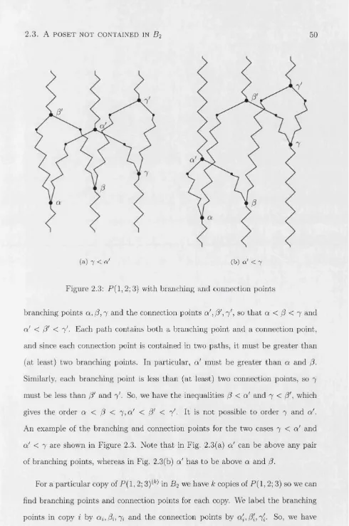
2.3 P ( l, 2; 3) with branching and connection p o i n t s ...50

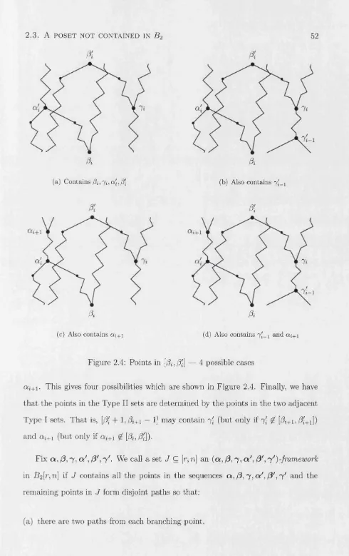
2.4 Points in [/?»,$] — 4 possible c a s e s ... 52

3.1 Forbidden induced suborders... 67

5.1 Counterexample to Conjecture 4 .4 ... 106

5.2 Counterexample to Conjecture 4 .4 ... 109

6.1 General counterexample for d(T) > 0,d(D[y]) = 0 ... 127

7.1 Subtrees of Ti and T2 ... 144

8.1 The two cases for Tb+ ... 154

(10)

8

(11)

9

A cknow ledgem ents

Firstly, I would like to thank Professor Graham Brightwell for his unfaltering super

vision. He introduced me to the problems studied here and he has been a constant

inspiration throughout my studies. I also extend my thanks to the whole of the

Mathematics Department at LSE. I have really appreciated the informal atmo

sphere around the department, and the friendly nature of all its members. I am sure

that this is owing, in part, to the informal workshops and discussions at the round

table—long may they continue. Particular thanks go to Dave Scott and Jackie Ev-

erid for their administrative support, Mark Baltovic for his IT expertise, and my

fellow research students for sharing the highlights and frustrations of research and

for our many conversations on a multitude of topics, a most welcome distraction.

Away from the university, my thanks go to all my friends living in and around

London who have made my time here such an enjoyable one. Special thanks go to

Owen Jones, Katrine Reimers and Esme Tarasewicz for being wonderful housemates,

and to Joe Walton and Nick Sample for their generosity and friendship.

My thanks, as always, to my parents and my brother, Matthew, for their loving

support and encouragement.

Finally, I thank the Engineering and Physical Sciences Research Council, the

London School of Economics and Political Science, and the Department of Mathe

matics for their financial support over the last four years.

(12)

10

S tatem en t o f originality

I declare that the work described in this thesis is wholly my own, except for the work

in Chapter 3. The work described in Chapter 3 was carried out in conjunction with

my supervisor, Professor Graham Brightwell and was worked on in equal proportion

by myself and Professor Brightwell.

Nicholas Georgiou (candidate)

s/s

(13)

11

Sum m ary

This thesis covers two areas in probabilistic combinatorics, specifically the com

binatorics of partially ordered sets. Problems and areas of study in probabilistic

combinatorics broadly fall into one of two classes. The first class contains prob

lems of a deterministic nature, which are particularly suited to some application of

probabilistic methods or techniques. The second class contains problems that are

themselves of a probabilistic nature. We cover problems from both classes.

In the first part of the thesis we investigate a family of random models of partial

orders, called classical sequential growth models. We study in detail the simplest

non-trivial model from the family and analyse the partial orders it produces. We

also study “continuum limits” of sequences of classical sequential growth models,

proving that particular sequences of these models do have continuum limits. We

also prove some results about the continuum limit of a general sequence of classical

sequential growth models, when it exists.

In the second part of the thesis we look at enumeration of embeddings of trees

into complete trees, which can be motivated by a partial-order variant of the best

secretary problem. We show that a monotone property of binary trees that was

conjectured to hold for arbitrary trees does not hold in general. We show that the

monotonicity on binary trees is an example of a correlation inequality on a certain

(14)

12

Part I

(15)

Pa r t I: Cl a s s i c a l s e q u e n t i a l g r o w t h m o d e l s 13

In this part we study a family of models of random partial orders, called classical

sequential growth models, introduced by Rideout and Sorkin [24]. These models

were proposed as possible models for discrete space-time, since they are the only

models satisfying certain desirable physical-looking conditions. In particular, we

will analyse the simplest non-trivial model from the family, and we will also define

and study a particular limit of a sequence of classical sequential growth models.

In Chapter 1 we give a full description of the family of models and a brief

summary of the results in [24], explaining the physical-looking conditions imposed

by Rideout and Sorkin, and noting that a particular model from the family can be

specified by a sequence of non-negative constants.

In Chapter 2 we study in detail the particular model called a random binary

growth model, showing that a random poset produced by the model almost surely

has infinite (poset) dimension. This shows that, despite the simple description of the

model, the random poset it produces has a complex structure. We give estimates for

bounds on the size of an up-set of a particular element and show that every element

in the random infinite poset is incomparable to only finitely many others. We also

present a specific poset that, with some positive probability, is not contained in the

random poset produced by the model. This contrasts the model with other random

models of partial orders, for example the random graph order, which contains any

specific poset almost surely.

In Chapter 3 we study the continuum limits of sequences of classical sequential

growth models. Rideout and Sorkin [25] have provided computational evidence

suggesting th at particular sequences of models have a continuum limit. We formalise

their results by defining what a continuum limit is, and we show that if a sequence

has a continuum limit then it must be an almost-semiorder. Using some results of

Pittel and Tungol [23] on random graph orders, we prove th at the continuum limit

of a sequence of random graph orders, when it exists, is a random semiorder. We

(16)

Pa r t I: Cl a s s i c a l s e q u e n t i a l g r o w t h m o d e l s 14

describes work carried out in conjunction with my supervisor, Professor Graham

(17)

15

C hapter 1

In trod u ction

We study a family of models of random partial orders, called classical sequential

growth models, introduced by Rideout and Sorkin [24]. Each model is defined on the (labelled) vertex set N, which we will always take to include 0. Any model can be

restricted to [n] = { 0 , 1 , 2 , , n} and regarded as a model of random finite posets. The model starts with a poset of one element (labelled 0), and grows in stages. At

stage n = 1 ,2 ,..., vertex n is added to the existing poset, Pn_i, by placing n above

some choice of vertices of Pn-i. The poset Pn is defined on vertex set [n] by taking

the transitive closure of the existing and added relations. This is called a transition

from Pn_i to Pn, written Pn_i —> Pn. The models are random, so each transition

occurs with some probability. These transition probabilities are fixed and depend

on the particular model. Let P(Pn- i —5> Pn) denote the probability of transition

Pn_i —►Pn occurring.

Rideout and Sorkin then impose four conditions on the transition probabilities,

with the aim of giving the model physical meaning. They call these conditions:

internal temporality, discrete general covariance, Bell causality and Markov sum.

The first and last conditions are implicit in the mathematical approach to random

partial orders, namely that the labelling of a poset is natural (can be extended

(18)

Ch a p t e r 1. In t r o d u c t i o n 16

(at each stage n and for any fixed Pn- i the sum of probabilities over all possible

transitions Pn_i —►Pn must be equal to 1). Discrete general covariance states that

the probability of producing a particular poset should not depend on the labelling

of the poset, th at is, given two different sequences of transitions, ( P i —►P i + l ) and

(Qi —►Qi+1) which produce the isomorphic posets Pn and Qn, the products

n—1 n—1

n P T i - P m ) and ^ P(Qi ^ Qi-\-1)

i= 0 i —0

must be equal. So, for example, discrete general covariance immediately implies

th at any two transitions from Pn_i to isomorphic posets Pn and P'n have the same

transition probability P(Pn- i —> Pn) = P(P»»-i —8►P'n)- Bell causality is a condition on ratios of transition probabilities. (Note that in [24] Rideout and Sorkin only

study “generic” models, meaning that all transition probabilities are non-zero, in

order to make sense of this condition.) Given a particular poset P , and any two

transitions P —» P ', P —* P" which add the new element n, let S be the set of all elements which are incomparable with n in both P r and P ". Let Q be the poset

formed from P by removing all the elements of S (and obsolete relations), and define

Q' and Q" similarly. Then, Bell causality states that

P (P -> P') P(Q -► Q')

P ( P _+ p //) “ P (Q Q //) ’

the idea being that, since the new element is not placed above any of the elements

of S in either transition, the presence of the set S should not affect the ratio of the transition probabilities.

A particular model is specified by a sequence t = (to» • • •) °f non-negative

constants. The random poset is defined as the transitive closure of a directed random

graph Gt on N in which all arcs go from a lower numbered vertex to a higher. The

arcs are selected sequentially, considering each vertex n in turn and choosing the set

Dn C [n — 1] of vertices sending an arc to n; the probability th at Dn is equal to a set D being proportional to t\D\, so that

P (A . = D) = .

(19)

A model defined according to this description is called a classical sequential

growth model Rideout and Sorkin show that these models are the only generic models satisfying their conditions. It is an easy exercise to check that these models

do indeed satisfy the four conditions; for example, Bell causality holds essentially

because the relative probability that element n selects a set D, defined as t\D\, is

independent of n.

Varadarajan and Rideout [31] and Dowker and Surya [12] have studied the sit

uation where the transition probabilities are allowed to be zero. The Bell causality

condition becomes a condition on products of transition probabilities and the type

of models th at satisfy the conditions are very similar to the generic models described

here.

The family of classical sequential growth models also contains models of random

graph orders. A random graph order Pn>p is defined as follows. The ground set of

Pn,p is the set { 0 ,1 ,..., n — 1}. For each pair of vertices i < j the relation (i , j) is introduced with probability p. The poset Pn>p is then the transitive closure of these relations. Random graph orders were introduced by Albert and Frieze [1] and

have been studied further by Bollobas and Brightwell [7, 8, 9] and Simon, Crippa

and Collenberg [27]. The area is covered in the survey of random partial orders by

Brightwell [10]. A classical sequential growth model defined by sequence t where

U = f for all i, and t = p /( 1 - p), will after stage n — 1 produce a random graph order Pn>p.

In the following chapter, we concentrate on the model where the sequence t is

(0 ,0 ,1 ,0 ,...), i.e., where all U are zero except 12. This means that \Dn\ = 2 for each

vertex n. We say that n selects the two vertices in Dn. So, in this model each vertex

n selects two vertices chosen uniformly at random from the set [n— 1]. We assume

that we start with the vertices 0 and 1 incomparable with probability 1 and then

add vertices n = 2 ,3 ,... according to the model. (So, for example, D2 = {0,1}

(20)

random poset it produces a random binary order.

This is the simplest interesting model; the model defined by t with t0 non-zero

and U equal to zero for i > 1 produces an infinite antichain (Dn = 0 with probability

1, for all n), and the model defined by t with to and t\ non-zero and U equal to zero for i > 2 produces a forest of infinitely many infinite trees, where each vertex is an upper cover of exactly one other vertex and a lower cover of infinitely many other

vertices. These are called the “dust universe” and “forest universe” , respectively, in

[24].

The random binary growth model also has potential applications in computer

science. Under the name of a random binary recursive circuit, the random binary

order has been studied by Mahmoud and Tsukiji [20, 21], Tsukiji and Xhafa [30] and

Arya, Golin and Mehlhorn [4]. These papers typically focus on the “depth” of the

circuit or the number of “outputs” of the circuit. These are considered as important

parameters in a computer science setting; however, they correspond to the height

of the random binary order and the number of maximal elements of the random

binary order, which are not particularly interesting parameters of a partial order.

Here we will consider parameters that are more interesting from a combinatorial

viewpoint, but these will probably not have useful analogues in the recursive circuit

formulation.

The random binary growth model is essentially the same as any other model

with f3 = = . .. = 0 since for large n the number of 2-element subsets of [n — 1] is significantly greater than the number of 1-element subsets and so the probability

of n selecting just one vertex (or no vertices) is very small in comparison to the

probability of n selecting two vertices. Therefore the results in the following chapter

(21)

19

C hapter 2

T h e random binary grow th m odel

Recall that the random binary growth model is defined as follows. Start with el

ements 0 and 1 incomparable; then each element n = 2 ,.. . selects two elements

uniformly at random from [n — 1], and we take the transitive closure. We will

restriction of B 2 to [ni, n 2\ = {x € N : rii < x < n2}.

The random binary order B 2 is a sparse order; each vertex n has at most 2 lower

covers since x is a lower cover of n if and only if it is selected by n and is not below

the other vertex y selected by n. This means the Hasse diagram of B 2[n] has at

most 2n edges. Also, as we now show, the expected width (i.e., the expected size of

the largest antichain) of B 2[n] increases with n. A vertex x in B 2[n] is maximal if and only if all vertices y = x + l , x + 2 ,... ,n do not select x, so

denote the random binary growth model by B2 and the random binary order it pro

duces by B 2. We write B 2[n\ for the restriction of B 2 to [n] and B 2[ni,n2] for the

n P(rr is maximal in B 2[n]) = J J

y —x + l

y — 2 x(x — 1)

and so the expected number of maximal elements is

n(n -I- l)(2n + 1) n ( n -1-1)

(22)

Ch a p t e r 2 . Th e r a n d o m b i n a r y g r o w t h m o d e l 20

(In fact, this is shown in [20], where Mahmoud and Tsukiji also show that the number

of maximal elements of B 2[n\ tends in distribution to a normal random variable with

mean n j3 and variance 4n/45.) The maximal elements form an antichain, so the

expected width of B 2[n] is at least (n + l)/3.

However, the number of minimal elements is always 2, since only 0 and 1 are

minimal. Moreover, the expected number of minimal elements of B 2[ni,n2], for

ni > 2, is bounded above by ni as n2 tends to infinity. Indeed, a vertex x in

B 2[ni,n2] is minimal if and only if it selects both vertices from [ni — 1], and the probability of this is (?2l) / (2) = n i(n i ~ l ) /x ( x — 1). Summing over x from n\ to

n 2 gives the expected number of minimal elements equal to n\ — n\{n\ — l ) / n 2.

In Section 2.1 we study the dimension of B 2. The dimension of a poset P

on ground set X is the minimum number of linear orders on the set X whose

intersection is equal to P. In other words, the minimum number of linear orders Li

such that x < y in P if and only if x < y in Li for all i. An equivalent definition

is th at the dimension of P is the smallest d such that P can be embedded into

R d, where R d is the d-dimensional Euclidean space with ordering (x i,...,X d ) <

( 2 / 1 , . . . ,yd) in R d if Xi < yi in R , for a l i i = 1 ,... ,d. (The equivalence can be

easily proven; the essential observation is that the linear orders on X correspond

to the coordinate-wise orderings of the embedded points in R d.) Since B 2 is sparse,

one might suppose there to be a relatively simple structure to B 2. However, we

show this is not the case in so much as showing th at B 2 has infinite dimension,

almost surely. Using standard notation (see, e.g., [29]), we write P (l,2 ;ra ) for the

subposet of the subset lattice formed by the 1-element and 2-element subsets of

the m-element set { l ,...,m } ordered by inclusion. Spencer [28] proved that the

dimension of P ( l, 2; m) is greater than log2log2m, so we show that B 2 has infinite

dimension, almost surely, by showing it contains a copy of P ( l, 2; m) as a subposet,

for each m, almost surely. This is done by counting (and bounding the expected

(23)

Ch a p t e r 2 . Th e r a n d o m b i n a r y g r o w t h m o d e l 21

directed random graph Gt ).

In Section 2.2 we study the sizes of up-sets in B 2[n] and, related to this, the

number of elements in B 2 incomparable with an arbitrary element. Although B2 is

sparse, we show th at for all r the number of elements incomparable with r is finite.

In particular, this implies that B 2 does not contain an infinite antichain, almost

surely. Moreover, for any classical sequential growth model defined by sequence t

where U ^ 0 for some i > 2, the same result is true, th at the random poset produced

does not contain an infinite antichain, almost surely.

We use the differential equation method of Wormald [32, 33] which specifies when

and how a discrete Markov process can be closely approximated by the solution to

a related differential equation. We prove a version of Wormald’s theorem which

makes explicit the errors in the approximation. We use this result to analyse the

growth of the up-set of an arbitrary point. For a fixed point r, write U^ for the set

of elements above r in the finite poset B2[n\. We can think of “growing the poset”

by increasing n. Then \UrU^\, which depends on n, can be considered as a Markov

process. Using this “differential equation method” , we give good estimates on \U^\

for particular values of n, and show that there exists an n = n(r) such that Ir C [n\.

Here, Ir is the set of vertices greater than r which are incomparable with r. So, for

fixed r, there are no vertices greater than n incomparable to r, and so the number

of vertices incomparable with r is finite. We provide two similar proofs, one giving

bounds for a typical r, and one giving bounds for all but finitely many r.

Is the fact th at P (l,2 ,m ) is almost surely contained in B 2 a special case of something more general? Is it possible, as in the case of random graph orders, that

every finite poset is contained in J52, almost surely? In Section 2.3 we show that this is not the case. We use our result from Section 2.2, that there is an n = n(r) such

that for all but finitely many r, there are no vertices greater than n incomparable

with r. So, we know that if two elements in B 2 have labels with a large enough

(24)

2 .1 . T h e d i m e n s i o n o f B 2 22

in B 2 must have two elements whose labels have large difference. Combining these

two results, we provide an example of a poset not contained in B 2 (or rather, there

is a positive probability that B 2 does not contain the poset).

2.1

T he dim ension o f

B

2

We write P ( l, 2; m) for the subposet of the subset lattice formed by the 1-element

and 2-element subsets of the set { 1 ,..., m} ordered by inclusion. For a particular

vertex r, let Ur be the set of all vertices above r in B 2 and let u fi be the set of all vertices above r in B 2[t]. Denote by 7* the hitting time of the event \Ur\ — k, i.e.,

the smallest t such that \U^\ = k, and the waiting time between events \Ur\ = k — 1

and \Ur\ = k by W*, so that Tk+i = Tk + Wk+1- We include the point r in Ur so

that T \ = r .

We now show that, for every m, there exists a copy of P (l,2 ;m ) in B 2, almost

surely. This is enough to show that B 2 almost surely has infinite dimension, since

dim P ( l, 2; m) > log2 log2 m (see [28]).

In fact, we will prove a stronger result, that for each m there exists an r0 such

that the probability of there being a copy of P ( l, 2; m) in B 2[r, 2r 7/5] is greater than

3/5 for all r > r$.

We use the following lemma to find a copy of P ( l, 2; m) in B 2[r, 2r 7/5].

L em m a 2.1. For any m, and any n\ < n 2, if we have sets X = { x i,... ,x m} C [721,722], Y = { y i, . .. ,t/m} Q [wi,n2], where M = (7J), and the following conditions hold

(i) the points in X are incomparable in B 2[ni,n2\,

(25)

then X U Y is a copy of P (l,2 ;ra ) in B 2[ni,n2] where X is the set of minimal elements and Y is the set of maximal elements.

Proof. Let < be the order on B 2[ni,n2]. To show that X U Y is a copy of P( 1,2; m)

we need to show that the only relations are those described by condition (ii). That

is, that there are no relations of the form Xi < Xj, yk < yi or yk < x it

By condition (i) there are no relations of the form Xi < Xj. So, suppose there exists some relation yk < yi. Since |T| = M = (™), condition (ii) implies that there exists a pair Xi, Xj with xj < yk. But then Xi, Xj < yi contradicting condition (ii).

Suppose there exists some relation yk < Xi. Then by condition (ii) there exists some

yi with Xi < yi. But then yk < yi which leads to a contradiction as above.

So, X U Y is a copy of P ( l, 2; m) and X is the set of minimal elements and Y is

the set of maximal elements. □

P roposition 2.2. For every m, there exists anro such that the probability of there being a copy of P( 1,2; m) in B 2[r, 2r 7/5] is greater than 3/5 for all r > ro.

Proof. We will prove the result as follows. Assume that m is fixed, ro is sufficiently large and r > ro- First we find a set of points that satisfies condition (i) of Lemma 2.1

with some high constant probability. Because of the sparsity of B 2, it is easy to find

this set. Here we will take the points r , r + l , . . . , r + m — 1. These points will form

the minimal elements of a copy of P ( l, 2; m). We then grow the poset up to size r 7/5,

keeping track of the sizes of the up-sets of these chosen minimal points. The value

r7/5 is chosen so that the up-sets are large enough, but their pairwise intersection is still an insignificant fraction of the whole up-set. This means that the set of points

above one and only one of the minimal points is reasonably large. The bulk of the

proof is in showing this. Finally, we grow the poset up to size 2r 7//5 to find the points

satisfying condition (ii) of Lemma 2.1. Indeed, we look for points in [r7/5 + 1,2r 7/5]

selecting a pair of points from each pair of “exclusive up-sets”. Because the sizes of

(26)

2 .1 . Th e d i m e n s i o n o f B 2 24

points is at least some constant probability. We then apply Lemma 2.1 to obtain

the result.

Following this scheme, where m is fixed, is sufficiently large and r > ro,

consider the points r, r + 1, . . . , r + m — 1. We attem pt to find a copy of P( 1,2; m)

in which these are the minimal elements. We have,

m' 1

0

P(r, r - f l , . . . , r + m —1 are incomparable) = TF+K ^ 9/10 for r 0 > i =1 V 2 J

20m2.

Now grow the poset by adding points up to n = r 7/5. We consider the growth

of the set Ur. We calculate the expected waiting time EWfc+i as follows. Suppose

Tfc = t, then since Wk+\ always takes integer values greater than or equal to 1 we have

oo oo j / t + l - k \

e w m = i + £ I W + 1

>i)

= i +

EII

j =1 j = l Z=1 V 2 /

and using the inequalities 1 — x < e~x and f ^ +1 }{x)dx < ]Cj=a f U ) — l a -i f ( x )dx i for / decreasing, we have

\ 2 - k '

oo J ( t + l - k \ O O / J / , . I

m.,-i+£nwsi+E n ( ^

_{j = l i = i} _{I 2}_J _{3=1 \ l = 1}_' + I

oo / 3

< l + ] T e x p ( - 2 ^ k t "f- I

j= 1 \ /=!

/ /*J

1 + exp y —2k J

r j + l i

< 1 + ^ exp ( —2k I -—jdl

j=i

. * + 1 \ 2fc

- 1 + (t +

1)2ti

(* + / + i ) 2^

(t + i ) 2* l

That is,

So, we have

E(Wk+1\Tk) < 1 +

(t + I)2*- 12 k - 1

Tfc + 1

2fc — 1

(27)

which by induction on k gives

E 7 i+ 1 < (227 ( 2fe))r- + 2fc. (2.2)

Using Stirling’s approximation we have

(2k \ y/2n(2k)2k+1/2e~2k+1/(24k+1) 2 2k+l/2el^ 24k+^

I I ^ ^ . TQr jj» ^ 1

\ k J - ( V2n kk+i/2e-fc+i/i2fc)2 - y / ^ k ^ e 1/ ^ ’ “ ’

so ETfc+i < v/7re1/6fc_1^24fe+1^v/fcr + 2fc, for k > 1. For k > 2 , y/^el^ k~l^ 24k+Vj < 2

and using (2.2) we have ET2 < 2r + 2, so ETk+i < 2r\/fc + 2/: and so

E T fc < 2r V k + 2fc. ( 2 . 3 )

If we similarly define Ur+i, T ^ \ W® for r + z, z = 1, . . . , m — 1 and write for

Tfc, then we have = r + i, giving equations

E 2 & < j F T it® 3 0 +)■ (2-4) E 3 & < (2*/C J))(r + i) + 2fe, (2.5)

ET’^i) < 2(r + i)\/fc + 2k, (2.6)

corresponding to equations (2.1),(2.2) and (2.3).

For r0 > m we have r + z < r + m < 2r, so (2.6) becomes

EjjW < 4r\/k + 2k, i = 0, . . . , m —1.

So, recalling th at n = r 7/5, we have

F{\Uln]\ < r 3/4) = P ( r r3/4 > n) < ETr 3/4/ n

< (4r11/8 + 2r3/4) / r7/5 < 6/ r1/40 < l /1 0m

for r0 > (60ra)40, and similarly for |£/”+i|, z = l , . . . , m — 1.

Therefore, P(all |c4"]| , . . . , It/i+L-il > r3/i) > 9/10.

We say a point x selects a pair of sets (Xi, X 2) if Dx = {oq, x 2} for some x\ G X \

(28)

bounds on we can show that, with high probability, there exist points in B2[2n]

selecting each pair (£/]+*, We might hope for these to form the maximal points

of a copy of P( 1,2; m), since for each pair of minimal points r + i, r + j we have a point above both. However, it is possible for these potential maximal points to be

above more than 2 minimal points. We need to find points above exactly 2 of the

minimal points. To do this we need to look at a subset of £/r+i, namely the set of

points above r + i but not above any other r + j for j ^ i.

For points x, y in B 2, write Uxy for the set of points above both x and y. Consider

the restricted poset B2[n] and write Uxy for the set of points in B2[n] above both x

and y. We will show that |C/^+1| is small in comparison to \uln^\ and | | - Call

a sequence of integers from [r,n] a path if ij selects ij-i in the poset, for

j = 2 , . . . , s. So a path is necessarily a strictly increasing sequence. We say a path (ij)j=i is from to is. Define a forked path with ends x, y, z and connection point

w to be three paths, one from x and one from y both to w, and a third from w to z

(so x, y < w < z), with w the only common point of the first two paths. Note that

we allow the possibility that w = z, in which case the third path is the single point

w — z.

For each point u in U^ + 1 there must be paths Pr from r to u and PT+\ from r + 1 to u\ if we set v = min{j : j is a common point of Pr and Pr+i} then by taking

the subpath (subsequence of consecutive terms of a path) from r to v (of Pr), the

subpath from r + 1 to v (of Pr+i) and the subpath from v to u (of either Pr or Pr+1) we have a forked path with ends r, r + 1 and u, and connection point v. This

forked path is not necessarily unique, since Pr and Pr + 1 are not necessarily unique.

Let F P ( r, r + 1, v) be the total number of forked paths with ends r and r + 1 and connection point v all fixed, and with arbitrary third end u, with v < u < n. Let

FP(r, r + 1) = Y^ ) = r + 2 F P{r,r + i, u). Then \Urr+i\ < F P ( r , r + 1).

Now, the probability that a strictly increasing sequence {ij)Sj= 1 is a path in B2[n]

(29)

We can also calculate the probability that the points {ioAi> • • • A«}Ao < h <

• • • < is form two disjoint paths in ^ [ n ], one from zq, the other from ii, as follows.

Start with two sequences A — (io) and B = (ii), then taking each point ij, j =

2, . . . ,s in turn make it the next term in either sequence A or sequence B. (So, the

resulting A and B are disjoint subsequences of (ij)J=0)- The probability that we

can make A and B paths is the probability that at each step ij selects one of the

current end terms of A or B. For step j this is at most 4/ij so by independence the

total probability is less than I I ^ ^ A j ) - We have inequality here because we are

over-counting the case where ij is above both of the current end terms of A and B.

The expected size of F P ( r ,r + l,v) is the sum over all subsets I of [r, n\,

with r, r + l , v E I, of the probability that I forms a forked path with ends

r, r + l , m a x / and connection point v. This is the probability th at I <v = {i £

I : i < v} forms two disjoint paths from r and r + 1; and v selects the end of both paths; and I>v = {i £ I : i > v} forms a path from v to m ax /. So, for I = {r, r + 1, z2, . •., ia-i, v, is+i ,... , i s+s'} with ij increasing and r + 1 < i2,

i < v < is+i this probability is less than YYj^f^/^j) X V ( 2 ) X 1 1,7=1 (^As+j)*

So the sum over all such subsets I can be written as the following product, since

the individual terms of the expanded product correspond exactly to the required

probabilities for all subsets /,

E" (",'+1'’)s,n ( 1+9 ® ,n ( 1+0

\ r + 1J v(v — 1) \ v J 2rf_

~ r4 ’

using the inequalities 1 + x < ex and S i= a /W — la- 1f ( x )^x f°r / decreasing, so

in particular X)i=o V* — ^°S ^ “ ^°S (a ~ -0

(30)

2 . 1 . T h e d i m e n s i o n o f B 2 28

E F P (r, r + 1) < 2r 1/5. The same method gives the same upper bound on the

expected size of Uxy for all pairs (x, y) in [r, r + m —l p ) so P(|E/,S"+i| — (1 0m2) r 1/5) <

1/5m? and P(all \Uxy \ < (10m2)r1/5) > 9/10.

Let A ^ be the set of points above r but not above r 4- 1, . . . , r + m — 1 m. B2[n),

then \ LCi* ^ir+i- Similarly define x G [r + l , r + m — 1], Then,

for r > r 0 > 400m6, we have (10m2) r1/ 5 < r3/4/2m so with probability greater than

4/5 we have all \ A^\, x G [r, r + m — 1] at least \ r z^ .

We grow the poset by adding a further n = r7/ 5 points, to find our maximal

points: M = (™) points a i , . . . , a M, so that each pair of sets ( A ^ ^ A y 1^), (x,y) G

[r, r + m — l p ) is selected by some a*.

Now,

I4^ll>dn] I r 3/2 r 3/2

P (n + i selects ( 4 ”1,4 "ii)) = ^ 2(n + i) 2 ~ f°r ’ “

SO

/ r 3 /2 \ n P(none of n + 1, . . . , 2n selects ( A ^ \ ^4j.+i)) < ( 1 — j

< exp(—r1//10/8),

which is less than 1/10M for r0 > (81oglOM)10. The same calculations give the

same upper bound on the probability of failing to find a point in [n + 1,2n] which

selects ( A & \ A $ ) for each (x,y) G [r, r + m — l p ) , so the probability of failing to find points a i , . . . , <zm in [n + 1,2n] as desired is less than 1/1 0.

So with probability at least 3/5 we have sets {r, r + 1, . . . , r + m — 1} and

{ai, a2, . . . , c l m} satisfying the conditions of Lemma 2.1. Therefore ( r , r + l , . . . , r +

m — 1, ai, a2, . . . , om} is a copy of P( 1,2; m) in B2[r, 2n]. □

T h e o re m 2.3. For every m there exists a copy o / P ( l , 2 ; m ) in B 2, almost surely.

(31)

To find a copy of P( l , 2; m) in B2 we split B2 into disjoint sets of the form B2[n\, n2\

as follows.

For z = 1 , 2 , . . . , let = 2rJ^i + 1. By Proposition 2.2 the probability of there

not being a copy of P( l , 2; r a) in B2[ri, 2rJ^5] is less than 2/5, for each i. The

probability of not finding a copy of P(l , 2; r a) in the infinite poset B2 is less than

the probability of not finding a copy of P ( l , 2 ; m) in every poset B2[ri,2rJ^5]. But

the sets P2[^,2rJ^5] are disjoint, so the events “not finding a copy of P( l , 2; ra) in

-^2^ , 2rJ^5]” are independent. Therefore the probability of not finding a copy of

P( l , 2; m) in the infinite poset B2 is zero, as required. □

Corollary 2.4. B2 has infinite dimension, almost surely.

Proof. This is immediate, since dim P( l , 2; m) > log2 log2m. □

This tells us that, almost surely, there is no finite d such that B2 can be embedded

into Rd, the d-dimensional Euclidean space with ordering (xl f . . . , x d) < ( p i ,. . ., yd)

in Rd if Xi < yi in R, for allz = 1 , . . . , d, as defined earlier. W hat can be said for embeddings into other partial orders? Since classical sequential growth models have

been proposed as possible models of discrete space-time it would be interesting to

know whether the partial orders they produce can be embedded into a d-dimensional

Minkowski space for some finite d.

The Minkowski space M d is defined as the partial order on Rd with ordering

(zo,. . . , x d-i) < (y0, . . . , Pd-i) in M d if y0 - x0 > yjY^ZliVi ~ %i) 2 in R. The

Minkowski dimension of a partial order P is the smallest d such that P can be

embedded into M d. It is known that a finite partial order P can be embedded into

Md + 1 if and only if P can be represented as a d-sphere order. A d-sphere order is

a partial order on a ground set of spheres in Rd, with the ordering on the spheres

given by (geometric) containment. For example, the partial order P( l , 2 ; m) can

always be represented as a 3-sphere order. This is a specific case of a result of

(32)

2 .2 . Up-s e t s o f v e r t i c e s in B 2 30

most 4, for all m.

We believe th at the random binary order B2 has infinite Minkowski dimension.

A proof of this result could follow the proof strategy of Theorem 2.3; find a family

of partial orders with arbitrarily large Minkowski dimension that are almost surely

contained in B 2. Unfortunately, the partial orders known to have large Minkowski

dimension are all significantly more complex than P(1,2; m). Given the complexity

of the proof of Proposition 2.2 it would be ambitious to attem pt a proof using this

strategy. Instead, we make the following conjecture.

C o n jec tu re 2.5. B2 has infinite Minkowski dimension, almost surely.

We justify the conjecture as follows. If the poset B2 has finite Minkowski dimen

sion, then it can be embedded into M d for some d. Since the model B2 produces the

poset B2 sequentially, this means that at each stage n the finite poset B2 [n] can be

embedded into M d. However, this seems unlikely since at each stage the element n

selects two existing elements at random, each pair of elements being equally likely

with no regard to the existing structure of the embedding of B 2[n — 1] in M d. It

seems more likely that the random nature of the model B2 is such that, for large

enough n, the poset B2[n] produced at stage n cannot be embedded into M d.

2.2

U p -sets o f vertices in

B

2

Brightwell [11] proved that, almost surely, each element of B2 is comparable with

all but finitely many others. This result is contained within what we prove here;

we need a more refined version, providing an estimate of the number of elements

in B2[n] that are incomparable with an element r, and an estimate of the largest

element incomparable with r. Recall that U^ is the up-set of r in B2 [n] and that

/JN = [r, n] \ Uln] is the set of points larger than r and incomparable with r. We

(33)

2 .2 . U p - s e t s o f v e r t i c e s in B 2 31

use these estimates to provide estimates of the size

In [32, 33], Wormald presented a theorem which describes when and how a dis

crete time Markov process can be approximated by the solution to a related differ

ential equation. However the approximation is only in terms of asymptotic bounds;

here we state and prove a version of the theorem which gives explicit expressions for

the approximation.

We begin with some definitions.

D efin itio n 2.6. A function / : R2 —► R satisfies a Lipschitz condition on a con

nected open set P C M2 if there exists a constant L > 0 with the property

|/( ^ i, 2/i) ~ f { x2,2 /2 )I < L(\x1- x 2\ + \ y i - 2/21) (2.7)

for all (xi,yi) and (£2,2/2) in 7?.

D efin itio n 2.7. For Y a real variable of a discrete time random process Go, G1, . . .

which depends on a scale parameter n, we write Y(t) for Y ( G t), and for a connected

set P C M 2 define the stopping time Xp = 7p(Y) to be the minimum t such that

(:t / n , Y { t ) / n) £ P .

D efin itio n 2.8. A sequence of random variables Yo,Y\,... is a martingale with

respect to a sequence of cr-algebras To C T \ C ... if, for all i,

(i) Yi is .^-measurable,

(ii) E|Yi| < 0 0,

(iii) E(Fi+i | Ti) = Yi almost surely.

If, instead of (iii), we have:

• E(Y+i I 3~i) < Yi almost surely, then (Yi) is a supermartingale with respect to

(*i).

(34)

2 . 2 . U p - s e t s o f v e r t i c e s in B 2 32

The following lemma will be used in the theorem and is a simple extension of

a martingale inequality, known as Azuma’s inequality [5], to supermartingales. We

omit the proof, which can be obtained by an obvious modification to the proof of

Azuma’s inequality.

Lemma 2.9. Let Yq,Yi, • • • be a supermartingale with respect to a sequence of

cr-algebras f 0 C f i C . . . with Tq trivial, and suppose Yq = 0 and |l^+i — Y i \ < c for i > 0 always. Then for all a > 0,

> ac) < exp (—o?/2i).

We are now in a position to state and prove our version of the theorem.

Theorem 2.10. Let Y be a real-valued function of the components of a discrete time Markov process {G^}t>o- Assume that V CM? is connected, closed and bounded and contains the set

{(0,2/) : P(y(0) = yn) ^ 0 for some non-negative integer n}

and

(i) for some constant (3,

\Y(t + l ) - Y ( t ) \ < p

always for t < Tp,

(ii) for some function f : M2 —► M which is Lipschitz with constant L on some bounded connected open set Vq containing V, and some constant X,

|E (y(f + 1) - Y(t)\Gt) ~ f ( t / n , Y ( t ) / n ) \ < X/n

for t < Tv ,

(35)

Let w = w(n) be a fixed integer-valued function with w — o(n). Then the following are true.

(a) For (0,y) E V the differential equation

has a unique solution y = y(x) in T> passing through y(0) = y, and which extends for some positive x past some point, at which x = a say, at the boundary of V;

(b) Writing i$ = mm{\Tx>/w\, [a n / w\ } and ki = iw, there exists some B > 0 such that

P(|K (t) - ny(t/n) \ > B i + (/3 + i ) w ) < 2ie~ 2 w 3 ^ 2

for all i = 0,1, . . . , io —1 and all t, ki < t < ki+i, and for i = io and ki0 < t <

min {Tz>,an}, where Bi = ( ( 1 + L w / n) 1 — 1 ) B w / L , and y(x) and a are as in (a) with y = Y(0)/n.

P ro o f. Following the proof in [32], we have part (a) from the theory of differential

equations. Let y(x) and a be as in part (a).

Let 0 < t < Tx> — w and let 0 < k < w. This implies th at t + k < Xp and so

€T>.

' n 1 n '

By (i), we have \Y(t + k + l) — Y ( t + k)\ < /?. Also, by (ii),

E ( Y ( t + k + l ) - Y ( t + k )\ G t+k) < f ( — , + +

-V n n J n

< f ( i t W \ + L ( t + \ Y ( t + * ) - Y m + ±

\ n n J \ n n ) n

< f ( - + L (w + Pw ) + A

— \ n ’ n J n

where the second inequality follows from (2.7). Writing g(n) for (L(w + j3w) + A)/n,

the inequality becomes

(36)

2 .2 . Up-s e t s o f v e r t i c e s in B2 3 4

Therefore, conditional on Gt ,

Y ( t + k ) ~ Y(t) - k f ( ~ , - kg(n) \ n n J

is a supermartingale in k with respect to the sequence of cr-fields generated by

Gt, . . . , Gt+W. The differences of the supermartingale are, by (i) and (iii), at most

/? + / ( - , + 9(n) < P + 7 + 9 {n). \ n n J

So, by Lemma 2.9, for all a > 0,

P(Y(t + w) - Y ( t ) - w f ( ^, - wg(n) > + 7 + g(n))) < e~a2/2w. (2.8)

The same argument with

Y ( t + k ) ~ Y(t) - k f ( ~ , + kg(n) \ n n J

a submartingale gives

P(Y (t + w) - Y(t) - w f +wg(n) < - a ( f i + 7 + g(n))) < e~a2/2w. (2.9)

Setting a = 2w2/ n and combining (2.8) and (2.9) gives

P (|Y ( t + w ) - Y ( t ) - w f (£, ^ ) | > 2(w'2/n)(P + i + g(n)) + wg(n)) < 2e~2w3/n*.

(2.1 0)

Now, define ki = iw, i — 0 , 1 , . . . , z0 where Zo = m in {[T p/ w \, [crn/w\}. We

show by induction that for each such z,

Pfly(fci) - y(ki/n)n\ > B<) < 2ie - 2“ > 2 (2.1 1)

where Bi = ((1 + L w / n) 1 — 1 ) B w / L for some B > 0.

The induction begins by the fact that y(0) = Y(0)/n. (Take y = Yifi)/n and

(37)

2 .2 . Up-s e t s o f v e r t i c e s in B 2 35

So, assume (2.1 1) is true for i. Write

Ai = Y{ki) - y{ki/n)n

A2 = Y ( k i+1) - Y(ki)

A3 = y(ki/n)n - y(ki+i/n)n

The inductive hypothesis (2.11) gives |j4i| < Bi with probability at least 1 —

2ie~2w3/n\ By (2.10) we have

\A2 - wf (k i / n ,Y ( ki ) / n ) \ < 2(w2/n)((3 + 7 + g(n)) +wg(n)

with probability at least 1 — 2e-2u;3/n2.

Since / satisfies the Lipschitz condition and (ki+i/n, Y{ki+\)/n) G V (because

ki+1 < Tp), we also have

\A3 +wy\k i/n )\ = \y(ki/n)n - y(ki+i /n )n + wy'(ki/n)\

= | —wy'(k/n) + wy'(ki/n)\ for some k, ki < k < ki+1

— w \ f ( k / n , y ( k / n ) ) — f ( k i /n , y ( k i / n ) ) \ since y is solution to (a)

< wL [w/n + |y(k/n) - y{ki/n) |] by (2.7)

< w L [ w / n + ( w / n )\ f ( k' /n , y(k'/n)) |] for some k', ki < k' < k

< w L [ w / n + (w/n)7] by (iii)

= L( 1 + 7)w2/ n

where we have used the Mean Value Theorem (twice, to get lines 2 and 5). So,

\y'{ki/n) - f ( k i /n , Y ( k i ) / n ) \ = \f{ki/n,y(ki/n)) - f ( k i /n , Y ( k i ) / n ) \ < L\Ai\/n

and so assuming |i4i| < Bi, we have

I * - | < M L L 2 V + +

(38)

So, we have

\Y(ki+i) ~ y(ki+i/n)n\ = \A\ + A2 + A^\

< Bi + 2(w2/n) ((3 + j + g(n)) + wg(n) + L( 1 + 7)w2/ n + BiLw /n

= [2(w2/n ) (/? + 7 + </(n)) + iu</(n) + L(1 + 7)u>2/n] + £*( 1 + Lw/n) (2.1 2)

with probability at least 1 — 2(i + l)e _2™3/n2.

There exists B > 0 with

2(w2/ri) (/? + 7 + #(n)) + wg(n) + L( 1 + ~f)w2/ n < B w 2/ n (2.13)

for all n, so the term on the right hand side of inequality (2.1 2) can be replaced

with Bi(1 + Lw/n) -f B w2/ n, which is exactly Bi+1. So we have (2.1 1) for i + 1.

Finally, fcj+i — ki = w and the variation in Y (t) when t changes by at most w is at most /3w, by (i), and as before \y(ti/n)n — y(t2/n)n\ is less than w\ f( t / n , y(t/ri))\

for some t, t\ < t < t2 and this is less than 7w. So

P (|F (t) - ny(t/n)\ > Bi + {(3 + 7)it;) < 2ze_2w 3/n 2

for all i = 0,1, . . . , io — 1 and all t, ki < t < ki+1, and for z = io and ki0 < t <

min {Tp,cra}. □

We can apply Theorem 2.10 to |C/Jn^| as follows. We take as the Markov process

the random binary growth model, and as the real-valued function the size of the

up-set of a fixed vertex r. We then find sets T> and Uq, a function / , and constants

P,X and 7 satisfying the assumptions of the theorem. We obtain the following

corollary, which shows fairly precisely how | \ grows as m goes from some initial

n to (cr + l)n, where cr is a large constant. Over this range, \ U ^ \ / n grows from a small value to a value near to 1.

Corollary 2.11. For fixed r and any n > r, if \ u l n^\ = c(n)n for c(n) an arbitrary

function of n, then

' \U[n(a+l)]\ a + 1

(39)

for any constants 0 < <5 < 1/3, c r >0.

P ro o f. Fix a vertex r in B2[n}. Let the Markov process {(7t}t>o be the random

binary growth model but starting at stage n, so that Gt corresponds to B 2[n + 1].

Let Y(t) be the size of the up-set of r in B2[n4-1], i.e., Y(t) = |C/rn+t^|. For any

constant a, define V as the region {(x, y) : 0 < x < a, 0 < y < x + 1}. The region

V contains the interval {(0,2/) : 0 < y < 1}, and since |c4n^| = c(n)n, we must

have c(n) < 1 for all n. So, V satisfies the assumption in Theorem 2.10, since it contains all points (0,c(n)) for n = 1,2, __ We now find a set Vo, a function / ,

and constants /?, A and 7 satisfying assumptions (i)-(iii).

Since Y(t) = \uln+t^\ < n + t we have Y ( t ) / n < t / n +1, and so (t / n , Y ( t ) / n ) G V

as long as t / n < cr. This implies Tx> = [crn\ + 1.

Let P = 1, then (i) holds since \ Y ( t + l ) — Y(t)\ = \uln+t+1^\ — \ uln+t^\ < 1 always

for t < an.

Let f ( x , y) = 2y/(x +1) — y2/ { x + l) 2. Let L = 2.1 and 7 = 1.1. The function /

is bounded on V by 1 (attained when y = z + l ) and is continuous over the boundary

of V, so there exists an open set V containing V on which / is bounded by 7 = 1.1.

Also, | | V / | | , the length of the gradient vector of / ( V / = (ff> §£))» is bounded on

V by 2 and is continuous over the boundary of V, so there exists an open set T>"

containing V on which ||V /|| is bounded by L = 2.1. But then

| / ( u ) - / ( v ) | < L | u - v | (2.14)

(40)

of the two sets So, (iii) holds, and (ii) holds with A = 1, since

E (y (i+ 1 ) - Y(t)\Gt) = 0 x P (y (f+ 1 ) = y (i)|G t) + 1 x P ( y ( t + 1 ) = Y{t) + l\Gt)

(n + t + 1 — Y(t))(n + t — Y(t)) (n + t + 1 )(n + 1)

2Y(t)(n + t + l ) - Y ( t ) ( Y ( t ) + l) (n + t + l)(n + t)

which differs from f ( t / n , Y ( t ) / n) by at most l / n for t < an.

Now Tp = \an\ + 1 and so Tp > an. So Theorem 2.10 gives the result (b) for

i = i0, t = a n, namely that, for some B > 0,

Also, i0 < a n / w, so B io = ((1 + L w / n)*° — 1) B w / L < BweLa/ L, and (2.15)

be-w(n) = o{n) and so using the particular values for L,/5, 7 and A, we can satisfy

In the proof of Proposition 2.2 we bounded the expectation of the hitting time

many points of B2, almost surely. In terms of Ir we have the following theorem.

P ( | y ( c r a ) - ny(a)\ > B io + 2.1tu) < 2z0e 2v}3/n2, (2.15)

Here y(x) is the solution to the differential equation

dx x + 1 (x + l) 2

dy = 2_ y_______y^_

with initial condition ?/(0) = c(n). This is a homogeneous equation with solution

comes

for some B > 0.

Choose 5 with 0 < S < 1/3 and set the arbitrary function w(n) to n2/3+5. Then

equation (2.13) with B = 21 and this gives the required result.

□

(41)

2 .2 . U p - s e t s o f v e r t i c e s in B2 39

T h eo rem 2.12. For any constants e,77 with 0 < e < 1/4 and 0 < 77 < 1 there exists

To such that for all r > T’o both \Ir\ < r 2+4e and Ir C [r, r 4+8e] hold with probability at least 1 — 77.

P roof. Assume that r is sufficiently large. As before, let Tk be the hitting time of event \Ur \ = k, in terms of the growth model, i.e., the smallest t such that \ufi\ = k.

As in (2.3), we have ETk < 2ry/k + 2k. So ETr2 < 4r2 and Markov’s inequality gives

p(|tfK l6/»7)ra]| < r 2^ = p ^ 2 > (1 6 /T 7 )r 2) < 77/4 (2.16)

so that with suitably high probability the size of the up-set, \Ur16^ r ^|, is at least fraction 77/16 of the size of the poset, (16/77)r2.

Set no = ( l6/r))r2. We can rewrite equation (2.16) as

F(\Ulno]\/n0 > 77/ I6) > 1 - 77/4. (2.17)

Assume we have \UrU°^\/no > 77/16. Let e be an arbitrary constant with 0 < e <

1/4. We will use Corollary 2.11 to show that as the size of the poset, 77, increases

from no to (cr + l)no, for some constant cr, the ratio \Ur^\/n also increases, to a

value that is at least 1 — e /2.

\ulno]\

C laim 2.1. There exists a constant cr0 (dependent on e andr}) such that i f >

no

77/ I6 then -r----r— > 1 — e/ 2 with probability at least 2<JonJ e~2no .

(cr0 + l)n 0

P ro o f of C laim 2.1. Suppose |t/ino^|/n0 > 77/ I6. Applying Corollary 2.11 with

n = no, c(n0) = 77/ I6 and 8 = 1 / 1 2 we have

|[4"°(‘,+l)]| <7 + 1 no{a + 1) <7 + I6 /7 7

for any a > 0. Set cr0 so that

+ 1

, . / = 1 — e/4 (2.19)

(42)

/ 1 0e21<7° + 2.1\ 1

and then for sufficiently large r, I ---—— ) —-tt < e/4. Combining this

\ ^0 + 1 J Uq

inequality with (2.18) and (2.19) and setting a = &q gives the result. □

Let M = (I6/77)(<7o + 1), so that (cro + 1 )n0 = M r2. We have shown that, with

suitably high probability, \ U ^ \ / n > 1 — s/2 for n = M r 2. We now show that

\Ur^\/n remains close to 1 for all larger n. That is, that |c4n^|/n > 1 — e for all

n > M r 2.

Let rii = M r 2, and 72* = (1 + e/2)i_1ni for i = 2 ,3 ,__

C laim 2.2. I f |c4n<V n* — 1 — £/% ^ ien

(a) \u i^\/n > 1 — e for n = rii + l,ni + 2, . . . and

(b) \ulni+1^\/ni+i > 1 — e/ 2 with probability at least 1 — en]^e~2ni/ .

P ro o f of C laim 2.2. Suppose we have \uln^\/ni > 1 — e /2.

For part (a) we use the fact that |t4n^| is increasing in n, so that

\uln]\ \ulni]\

_

\ulni]\

> 1 -g/2 >

n 1 ( 1 + e /2)ui 1 + e/ 2

for all n = 72* + 1,72* + 2, . . . , [ra*+ij •

For part (b) we apply Corollary 2.11 with n — ni, cr = e/2 and 5 = 1/12. We have

l ^ / 2 + U l i e / 2 + 1 / i o e^ + 2.1\ l L IM-!,!/*

e /2 + 1 ) n ^ ) - n i t

(2.2 0)

72*(e/2 + 1) e/2 + l/c(jii)

with c(rii) > 1 — e /2. So,

e/ 2 + 1 ^ e/ 2 + 1

e/ 2 + l/c(n*) “ e/ 2 + 1/(1 - e /2) <

Random structures for partially ordered sets