http://dx.doi.org/10.4236/am.2015.66086
Degree Splitting of Root Square Mean
Graphs
S. S. Sandhya
1, S. Somasundaram
2, S. Anusa
31Department of Mathematics, Sree Ayyappa College for Women, Chunkankadai, India 2Department of Mathematics, Manonmaniam Sundaranar University, Tirunelveli, India
3Department of Mathematics, Arunachala College of Engineering for Women, Vellichanthai, India
Email: anu12343s@gmail.com
Received 15 April 2015; accepted 30 May 2015; published 2 June 2015
Copyright © 2015 by authors and Scientific Research Publishing Inc.
This work is licensed under the Creative Commons Attribution International License (CC BY).
http://creativecommons.org/licenses/by/4.0/
Abstract
Let f V G:
( ) {
→ 1, 2,,q+1}
be an injective function. For a vertex labeling f, the induced edgelabeling f∗
(
e=uv)
is defined by,(
)
( )
( )
2 2
2
f u f v
f∗ e=uv = + or
( )
( )
;
2 2
2
f u + f v
then,
the edge labels are distinct and are from
{
1, 2,, q}
. Then f is called a root square mean labeling ofG. In this paper, we prove root square mean labeling of some degree splitting graphs.
Keywords
Graph, Path, Cycle, Degree Splitting Graphs, Root Square Mean Graphs, Union of Graphs
1. Introduction
The graphs considered here are simple, finite and undirected. Let V G
( )
denote the vertex set and E G( )
de-note the edge set of G. For detailed survey of graph labeling we refer to Gallian [1]. For all other standard ter-minology and notations we follow Harary [2]. The concept of mean labeling on degree splitting graph was in-troduced in [3]. Motivated by the authors we study the root square mean labeling on degree splitting graphs. Root square mean labeling was introduced in [4] and the root square mean labeling of some standard graphs was proved in [5]-[11]. The definitions and theorems are useful for our present study.each edge e=uv is labeled with
(
)
( )
( )
2 2
2 f u f v f e uv
+
= =
or
( )
( )
2 2
2 f u f v
+
, then the edge
labels are distinct and are from
{
1, 2,,q}
. In this case f is called root square mean labeling of G.Definition 1.2: A walk in which u u1 2un are distinct is called a path. A path on n vertices is denoted by
n P .
Definition 1.3: A closed path is called a cycle. A cycle on n vertices is denoted by Cn.
Definition 1.4: Let G=
(
V E,)
be a graph with V =S1 S2 St T, where each Si is a set of vertices having at least two vertices and having the same degree and T= −V Si. The degree splitting graph of G is denoted by DS G( )
and is obtained from G by adding the vertices w w1, 2,,wt and joining wi to each vertex of Si,1≤ ≤i t. The graph G and its degree splitting graph DS G( )
are given inFigure 1.Definition 1.5: The union of two graphs G1=
(
V E1, 1)
and G2 =(
V E2, 2)
is a graph G=G1G2 with vertex set V =V1V2 and the edge set E=E1E2.Theorem 1.6: Any path is a root square mean graph. Theorem 1.7: Any cycle is a root square mean graph.
2. Main Results
Theorem 2.1: nDS P
( )
3 is a root square mean graph. Proof: The graph DS P( )
3 is shown inFigure 2. [image:2.595.80.540.81.128.2]Let G=nDS P
( )
3 . Let the vertex set of G be V =V1 V2 Vn where Vi={
v v v w1i, 2i, 3i, i,1≤ ≤i n}
. De-fine a function f V G:( ) {
→ 1, 2,,q+1}
byFigure 1. The graph G and its degree splitting graph DS G
( )
. [image:2.595.103.528.363.733.2]( )
1 4 3, 1 if v = −i ≤ ≤i n
( )
2 4 2, 1 if v = −i ≤ ≤i n
( )
3 4 1, 1 if v = −i ≤ ≤i n
( )
i 4 , 1f w = i ≤ ≤i n
Then the edges are labeled as
( )
1 2 4 3, 1 1i i
f v v = −i ≤ ≤ −i n
( )
2 3 4 1, 1 1i i
f v v = −i ≤ ≤ −i n
( )
1 4 2, 1 2i i
f v w = −i ≤ ≤ −i n
( )
3 4 , 1 2i i
f v w = i ≤ ≤ −i n
Then the edge labels are distinct and are from
{
1, 2,,q}
. Hence by definition 1.1, G is a root square mean graph.Example 2.2: Root square mean labeling of 4DS P
( )
3 is shown inFigure 3. Theorem 2.3:4DS P( )
4 is a root square mean graph.Proof: The graph DS P
( )
4 is shown inFigure 4. [image:3.595.153.479.378.733.2]Let G=nDS P
( )
3 . Let the vertex set of G be V =V1 V2 Vn where Vi={
v v v v w w1i, 2i, i3, 4i, 1i, 2i,1≤ ≤i n}
. Define a function f V G:( ) {
→ 1, 2,,q+1}
byFigure 3. Root square mean labeling of 4DS P
( )
3 .( )
1 7 5, 1 if v = −i ≤ ≤i n
( )
2 7 3, 1 if v = −i ≤ ≤i n
( )
3 7 1, 1 if v = −i ≤ ≤i n
( )
4 7 4, 1 if v = −i ≤ ≤i n
( )
1 7 6, 1i
f w = −i ≤ ≤i n
( )
2 7 , 1 if w = i ≤ ≤i n
Then the edges are labeled as
( )
1 2 7 4, 1 i if v v = −i ≤ ≤i n
( )
2 3 7 2, 1 i if v v = −i ≤ ≤i n
( )
3 4 7 3, 1 i if v v = −i ≤ ≤i n
( )
1 1 7 6, 1 i if v w = −i ≤ ≤i n
( )
1 4 7 5, 1i i
f w v = −i ≤ ≤i n
( )
2 2 7 1, 1 i if v w = −i ≤ ≤i n
( )
3 2 7 , 1 i if v w = i ≤ ≤i n
Then the edge labels are distinct and are from
{
1, 2,,q}
. Hence by definition 1.1, G is a root square mean graph.Example 2.4: Root square mean labeling of 4DS P
( )
3 is shown inFigure 5. Theorem 2.5: nDS P(
2K1)
is a root square mean graph.Proof: The graph DS P
(
2K1)
is shown inFigure 6.Let G=nDS P
(
2K1)
. Let the vertex set of G be V =V1 V2 Vn where{
1, 2, 3, 4, 1, 2,1}
i i i i i i i
V = v v v v w w ≤ ≤i n . Define a function f V G:
( ) {
→ 1, 2,,q+1}
by [image:4.595.135.477.472.701.2]Figure 6.The graph DS P
(
2K1)
.( )
1 7 5, 1 if v = −i ≤ ≤i n
( )
2 7 4, 1 if v = −i ≤ ≤i n
( )
3 7 2, 1 if v = −i ≤ ≤i n
( )
4 7 1, 1 if v = −i ≤ ≤i n
( )
1 7 6, 1i
f w = −i ≤ ≤i n
( )
2 7 , 1 if w = i ≤ ≤i n
Then the edges are labeled as
( )
1 3 7 4, 1 i if v v = −i ≤ ≤i n
( )
3 4 7 2, 1 i if v v = −i ≤ ≤i n
( )
4 2 7 3, 1 i if v v = −i ≤ ≤i n
( )
1 1 7 6, 1 i if v w = −i ≤ ≤i n
( )
2 1 7 5, 1i i
f v w = −i ≤ ≤i n
( )
3 2 7 1, 1 i if v w = −i ≤ ≤i n
( )
4 2 7 , 1 i if v w = i ≤ ≤i n
Then the edge labels are distinct and are from
{
1, 2,,q}
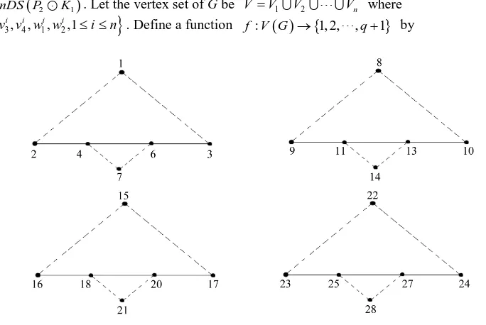
. Hence by definition 1.1, G is a root square mean graph.Example 2.6: The labeling pattern of 4DS P
(
2K1)
is shown inFigure 7. Theorem 2.7:nDS P(
2K2)
is a root square mean graph.Proof: The graph DS P
(
2K2)
is shown inFigure 8.Let G=nDS P
(
2K2)
. Let the vertex set of G be V =V1 V2 Vn where{
1, 2, 3, 4, 5, 6, 1, 2,1}
i i i i i i i i i
V = v v v v v v w w ≤ ≤i n . Define a function f V G:
( ) {
→ 1, 2,,q+1}
by( )
1 11 5, 1 if v = i− ≤ ≤i n
( )
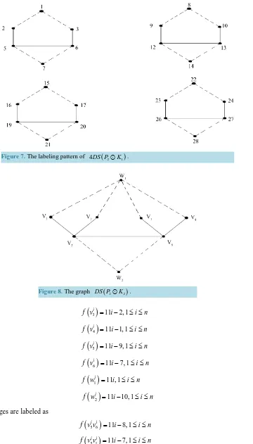
2 11 3, 1 i [image:5.595.237.394.84.237.2]Figure 7. The labeling pattern of 4DS P
(
2K1)
.Figure 8. The graph DS P
(
2K2)
.( )
3 11 2, 1 if v = i− ≤ ≤i n
( )
4 11 1, 1 if v = i− ≤ ≤i n
( )
5 11 9, 1 if v = i− ≤ ≤i n
( )
6 11 7, 1 if v = i− ≤ ≤i n
( )
1 11 , 1 if w = i ≤ ≤i n
( )
2 11 10, 1 if w = i− ≤ ≤i n
Then the edges are labeled as
( )
5 6 11 8, 1 i if v v = i− ≤ ≤i n
( )
5 1 11 7, 1 i i( )
5 2 11 6, 1 i if v v = i− ≤ ≤i n
( )
6 3 11 5, 1 i if v v = i− ≤ ≤i n
( )
6 4 11 4, 1 i if v v = i− ≤ ≤i n
( )
1 1 11 3, 1 i if v w = i− ≤ ≤i n
( )
2 1 11 2, 1 i if v w = i− ≤ ≤i n
( )
3 1 11 1, 1 i if v w = i− ≤ ≤i n
( )
4 1 11 , 1 i if v w = i ≤ ≤i n
( )
5 2 11 10, 1 i if v w = i− ≤ ≤i n
( )
6 2 11 9, 1 i if v w = i− ≤ ≤i n
Then the edge labels are distinct and are from
{
1, 2,,q}
. Hence by definition 1.1, G is a root square mean graph.Example 2.8: The labeling pattern of 2DS P
(
2K2)
is shown inFigure 9. Theorem 2.9: nDS P(
2K3)
is a root square mean graph.Proof: The graph DS P
(
2K3)
is shown inFigure 10.Let G=nDS P
(
2K3)
. Let the vertex set of G be V =V1 V2 Vn where{
1, 2, 3, 4, 5, 6, 7, 8, 1, 2,1}
i i i i i i i i i i i
V = v v v v v v v v w w ≤ ≤i n .
Define a function f V G:
( ) {
→ 1, 2,,q+1}
by( )
1 15 11, 1 if v = i− ≤ ≤i n
( )
2 15 8, 1 if v = i− ≤ ≤i n
( )
3 15 6, 1 if v = i− ≤ ≤i n
( )
4 15 5, 1 if v = i− ≤ ≤i n
( )
5 15 3, 1 if v = i− ≤ ≤i n
( )
6 15 2, 1 if v = i− ≤ ≤i n
( )
1 15 , 1 if w = i ≤ ≤i n
( )
2 15 14, 1 if w = i− ≤ ≤i n
( )
7 15 13, 1 if v = i− ≤ ≤i n
( )
8 15 12, 1 if v = i− ≤ ≤i n
Then the edges are labeled as
( )
7 1 15 11, 1 i if v v = i− ≤ ≤i n
( )
7 2 15 10, 1 i if v v = i− ≤ ≤i n
( )
7 3 15 9, 1 i iFigure 9.The labeling pattern of 2DS P
(
2K2)
.Figure 10. The graph DS P
(
2K3)
.( )
8 4 15 8, 1 i if v v = i− ≤ ≤i n
( )
8 5 15 7, 1 i if v v = i− ≤ ≤i n
( )
8 6 15 6, 1 i if v v = i− ≤ ≤i n
( )
7 2 15 14, 1 i if v w = i− ≤ ≤i n
( )
8 2 15 13, 1 i if v w = i− ≤ ≤i n
( )
1 1 15 5, 1 i if v w = i− ≤ ≤i n
( )
2 1 15 4, 1 i if v w = i− ≤ ≤i n
( )
3 1 15 3, 1 i if v w = i− ≤ ≤i n
( )
4 1 15 2, 1 i if v w = i− ≤ ≤i n
( )
5 1 15 1, 1 i if v w = i− ≤ ≤i n
( )
6 1 15 , 1 i if v w = i ≤ ≤i n
( )
7 8 15 12, 1 i i [image:8.595.105.523.83.237.2]Then the edge labels are distinct and are from
{
1, 2,,q}
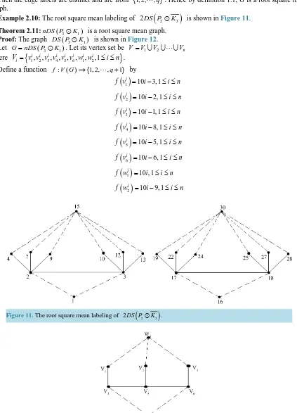
. Hence by definition 1.1, G is a root square mean graph.Example 2.10: The root square mean labeling of 2DS P
(
2K3)
is shown inFigure 11.Theorem 2.11:nDS P
(
3K1)
is a root square mean graph. Proof: The graph DS P(
3K1)
is shown inFigure 12.Let G=nDS P
(
3K1)
. Let its vertex set be V =V1 V2 Vnwhere Vi =
{
v v v v v v w w1i, 2i, 3i, 4i, 5i, 6i, 1i, 2i,1≤ ≤i n}
.Define a function f V G:
( ) {
→ 1, 2,,q+1}
by( )
1 10 3, 1 if v = i− ≤ ≤i n
( )
2 10 2, 1 if v = i− ≤ ≤i n
( )
3 10 1, 1 if v = i− ≤ ≤i n
( )
4 10 8, 1 if v = i− ≤ ≤i n
( )
5 10 5, 1 if v = i− ≤ ≤i n
( )
6 10 6, 1 if v = i− ≤ ≤i n
( )
1 10 , 1 if w = i ≤ ≤i n
( )
2 10 9, 1i
[image:9.595.100.523.92.679.2]f w = i− ≤ ≤i n
Figure 11. The root square mean labeling of 2DS P
(
2K3)
.Then the edges are labeled as
( )
4 1 10 5, 1 i if v v = i− ≤ ≤i n
( )
5 2 10 4, 1 i if v v = i− ≤ ≤i n
( )
6 3 10 3, 1 i if v v = i− ≤ ≤i n
( )
1 1 10 2, 1 i if v w = i− ≤ ≤i n
( )
2 1 10 1, 1 i if v w = i− ≤ ≤i n
( )
3 1 10 , 1 i if v w = i ≤ ≤i n
( )
4 2 10 9, 1i i
f v w = i− ≤ ≤i n
( )
6 2 10 8, 1 i if v w = i− ≤ ≤i n
Then the edge labels are distinct and are from
{
1, 2,,q}
. Hence by definition 1.1, G is a root square mean graph.Example 2.12: The labeling pattern of 3DS P
(
3K1)
is shown inFigure 13. Theorem 2.13: nDS K( )
1,3 is a root square mean graph. [image:10.595.137.493.312.726.2]Proof: The graph DS K
( )
1,3 is shown inFigure 14.Figure 13. The labeling pattern of 3DS P
(
3K1)
.Let G=nDS K
( )
1,3 . Let its vertex set be V =V1 V2 Vn where Vi={
v v v v w1i, 2i, 3i, 4i, i,1≤ ≤i n}
.Define a function f V G:
( ) {
→ 1, 2,,q+1}
by( )
1 6 5, 1 if v = −i ≤ ≤i n
( )
2 6 4, 1 if v = −i ≤ ≤i n
( )
3 6 2, 1 if v = −i ≤ ≤i n
( )
4 6 1, 1 if v = −i ≤ ≤i n
( )
i 6 , 1 f w = i ≤ ≤i nThen the edges are labeled as
( )
1 2 6 5, 1 i if v v = −i ≤ ≤i n
( )
1 3 6 4, 1 i if v v = −i ≤ ≤i n
( )
1 4 6 3, 1 i if v v = −i ≤ ≤i n
( )
2 6 2, 1i i
f v w = −i ≤ ≤i n
( )
3 6 1, 1i i
f v w = −i ≤ ≤i n
( )
4 6 , 1 i if v w = i ≤ ≤i n
Then the edge labels are distinct and are from
{
1, 2,,q}
. Hence by definition 1.1, G is a root square mean graph.Example 2.14: The labeling pattern of 4DS K
( )
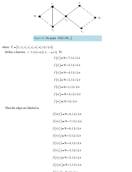
1,3 is shown inFigure 15. Theorem 2.15: nDS C(
3OˆK1,2)
is a root square mean graph.Proof: The graph DS C
(
3OˆK1,2)
is shown inFigure 16. [image:11.595.133.481.489.709.2]Let G=nDS C
(
3OˆK1,2)
. Let its vertex set be V =V1 V2 VnFigure 16.The graph DS C
(
3OˆK1,2)
.where Vi=
{
v v v v v w w1i, 2i, 3i, 4i, 5i, 1i, 2i,1≤ ≤i n}
.Define a function f V G:
( ) {
→ 1, 2,,q+1}
by( )
1 9 7, 1 if v = −i ≤ ≤i n
( )
2 9 5, 1 if v = −i ≤ ≤i n
( )
3 9 4, 1 if v = −i ≤ ≤i n
( )
4 9 2, 1 if v = −i ≤ ≤i n
( )
5 9 1, 1 if v = −i ≤ ≤i n
( )
1 9 8, 1i
f w = −i ≤ ≤i n
( )
2 9 , 1 if w = i ≤ ≤i n
Then the edges are labeled as
( )
1 1 9 8, 1 i if w v = −i ≤ ≤i n
( )
1 2 9 7, 1i i
f w v = −i ≤ ≤i n
( )
1 2 9 6, 1 i if v v = −i ≤ ≤i n
( )
1 3 9 5, 1 i if v v = −i ≤ ≤i n
( )
2 3 9 4, 1 i if v v = −i ≤ ≤i n
( )
3 4 9 3, 1 i if v v = −i ≤ ≤i n
( )
3 5 9 2, 1 i if v v = −i ≤ ≤i n
( )
4 2 9 1, 1 i if v w = −i ≤ ≤i n
( )
5 2 9 , 1 i if v w = i ≤ ≤i n
Figure 17.The root square mean labeling of 4DS C
(
3OˆK1,2)
.Example 2.16: The root square mean labeling of 4DS C
(
3OˆK1,2)
is given inFigure 17.References
[1] Gallian, J.A. (2012) A Dynamic Survey of Graph Labeling. The Electronic Journal of Combinatories. [2] Harary, F. (1988) Graph Theory. Narosa Publishing House Reading, New Delhi.
[3] Sandhya, S.S., Jayasekaran, C. and Raj, C.D. (2013) Harmonic Mean Labeling of Degree Splitting Graphs. Bulletin of Pure and Applied Sciences, 32E, 99-112.
[4] Sandhya, S.S., Somasundaram, S. and Anusa, S. (2014) Root Square Mean Labeling of Graphs. International Journal of Contemporary Mathematical Sciences, 9, 667-676.
[5] Sandhya, S.S., Somasundaram, S. and Anusa, S. (2015) Some More Results on Root Square Mean Graphs. Journal of Mathematics Research, 7.
[6] Sandhya, S.S., Somasundaram, S. and Anusa, S. (2014) Root Square Mean Labeling of Some New Disconnected Graphs. International Journal of Mathematics Trends and Technology, 15, 85-92.
http://dx.doi.org/10.14445/22315373/IJMTT-V15P511
[7] Sandhya, S.S., Somasundaram, S. and Anusa, S. (2014) Root Square Mean Labeling of Subdivision of Some More Graphs. International Journal of Mathematics Research, 6, 253-266.
[8] Sandhya, S.S., Somasundaram, S. and Anusa, S. (2014) Some New Results on Root Square Mean Labeling. Interna-tional Journal of Mathematical Archive, 5, 130-135.
[9] Sandhya, S.S., Somasundaram, S. and Anusa, S. (2015) Root Square Mean Labeling of Subdivision of Some Graphs.
Global Journal of Theoretical and Applied Mathematics Sciences, 5, 1-11.
[10] Sandhya, S.S., Somasundaram, S. and Anusa, S. (2015) Root Square Mean Labeling of Some More Disconnected Graphs. International Mathematical Forum, 10, 25-34.