Munich Personal RePEc Archive
Genetic Algorithm Optimisation for
Finance and Investments
Pereira, Robert
February 2000
Online at
https://mpra.ub.uni-muenchen.de/8610/
School of Business
Genetic Algorithm Optimisation for Finance and Investment
DISCUSSION PAPERS
Robert Pereira
Series A
00.02 February 2000
The copyright associated with this Discussion Paper resides with the author(s)
Genetic Algorithm Optimisation for Finance
and Investment
Robert Pereira
Department of Economics and Finance
La Trobe University
Bundoora, Victoria, Australia, 3083
phone: (613) 9479 2318
fax: (613) 9479 1654
r.pereira@latrobe.edu.au
February 2000
Abstract
This paper provides an introduction to the use of genetic algo-rithms for financial optimisation. The aim is to give the reader a basic understanding of the computational aspects of these algorithms and how they can be applied to decision making in finance and investment. Genetic algorithms are especially suitable for complex problems char-actised by large solution spaces, multiple optima, nondifferentiability of the objective function, and other irregular features. The mechan-ics of constructing and using a genetic algorithm for optimisation are illustrated through a simple example.
1
Introduction
see Trippi and Turbin (1996), Deboeck (1994), and Weigend, Abu-Mostafa and Refenes (1997).
Computers are considered important in developing trading strategies, fi-nancial analysis and portfolio optimisation because humans have limited cog-nitive ability and can be inconsistent in decision making; see Kahneman and Tversky (1982). By using computers, numerous alternative trading strate-gies, financial scenarios or portfolios can be developed and quickly appraised. However, Bauer and Liepens (1992) argue that given a seemingly limitless number of different combinations, even computers are severely limited in terms of an exhaustive search. Genetic algorithms provide one method for the rapid evaluation of real-time financial and investment possibilities, which is important in today’s fast paced and dynamic financial environment.
Genetic algorithms, developed by Holland (1975), are a class of adaptive search and optimisation techniques.1
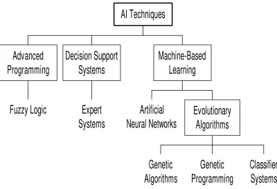
These algorithms are extremely efficient at searching large solution spaces. Furthermore, Dorsey and Mayer (1995) have shown that a genetic algorithm is a robust or effective method for opti-misation of complex problems characterised by multiple optima, nondifferen-tiability, and other irregular features. Unlike other optimisation techniques, such as gradient-based methods which solve for the optimal value using an analytical approach, genetic algorithms use an iterative numerical approach. Genetic algorithms are a form of artificial intelligence, which is based on the idea of simulating human-like decision making ability using a com-puter. Artificial intelligence techniques can be grouped succinctly into the three broad areas of advanced programming techniques, decision support and expert systems, and machine-based learning techniques as shown in Figure 1. Genetic algorithms belong to the class of evolutionary algorithms, which attempt to solve difficult problems by evolving an initial set of potential so-lutions into better soso-lutions through an iterative process. This is achieved through a process referred to as natural selection or survival of the fittest, which is based on Charles Darwin’s theory of evolution.
[Insert Figure 1.]
Both evolutionary algorithms and neural networks are machine-based learning techniques, where the latter attempt to learn patterns or relation-ships usually from large samples of data. These techniques can be employed to develop and optimise trading rules, forecast financial asset returns, or con-struct optimal portfolios. Since a large part of the literature consists of neural
1
network applications, this paper will focus exclusively on genetic algorithms and their role in financial optimisation.
This paper is organised as follows. Section 2 describes the mathematical structure and operations involved in using a genetic algorithm. Section 3 considers a simple example to illustrate the procedure involved in deriving a solution for a simple optimisation problem using a genetic algorithm. The advantages and disadvantages of this technique in relation to other optimi-sation methods are given in Section 4. Section 5 outlines previous studies which have applied genetic algorithms to finance and investment. Finally, Section 6 provides a summary of the paper.
2
Mathematical structure and operations
Typically, any genetic algorithm used for the purpose of optimisation consists of the following features:
1. binary representation, 2. objective function,
3. genetic operations (selection, crossover and mutation).
2.1
Binary representation
In order to solve an optimisation problem using a genetic algorithm, poten-tial solutions or candidates are usually represented by vectors consisting of binary digits or bits.2
In general, the binary representation of an individual candidate is given by
x= [x1, x2, x3, ..., xb] (1)
where the value of each of the b elements is either a zero or one. This repre-sentation is based on the binary number system. Thus a particular candidate with a binary representationxi has a corresponding decimal equivalent value
given by
2
yi = b
X
j=1
(2n−j
)xj (2)
where the elements xj of vector xi are the different values of the binary
representation with a value of either zero or one.3
For example, a candidate with a binary representation given by
xi = [0 1 0 0 1]
has a decimal equivalent value given by
yi = (2 4
×0) + (23×1) + (22×0) + (21×0) + (20×1) = 8 + 1 = 9
which is equal to a corresponding decimal value of nine.
2.2
Objective function
Ultimately the goal of a genetic algorithm is to find a solution to a complex optimisation problem, which is optimal or near-optimal, quickly and at lowest cost. This property is important for short-term trading, for example arbi-trage or market making operations. In these cases, obtaining a near-optimal solution relatively quickly is more important than obtaining the optimal so-lution at the cost of a significantly greater amount of time. In order to do this a genetic algorithm searches for better performing candidates, where performance can be measured in terms of an objective function.
The objective function used in a genetic algorithm can be expressed as
z =F(y,W) (3) where the vector y consists of decimal equivalent values, each with a cor-responding binary representation given by x, and W is a set of other pa-rameters or variables which are not directly of interest. In terms of finan-cial market problems, the objective function could be represented by profit.
3
Specifically, the objective could be to maximise trading profits by choosing the appropriate parameter values for a particular trading rule given a sample of financial market data. Another financial problem, could involve optimal portfolio selection, where the objective is to choose the proportion of financial assets to hold in a portfolio such that risk is minimised given the constraint of achieving a specified level of return.
Each candidate’s performance can be assessed using the objective func-tion given by Equafunc-tion 3. For example the decimal equivalent value of a particular candidate given by yi has a performance value of F(yi). The
ob-jective function is extremely important in guiding the genetic algorithm in its search for the optimal solution; this is discussed further in Section 4.
2.3
Genetic operations
The search process employed by a genetic algorithm is driven by three im-portant operations:
1. selection, 2. crossover, 3. mutation.
It is through these genetic or biological operations that an initial pop-ulation of randomly generated candidates to a problem is evolved through successive iterations, referred to as generations, into a final population con-sisting of the optimal or a near-optimal solution.4
These operations can be thought of as an effective procedure for updating the candidates’ solution values from one iteration to the next. The search procedure which ensues is highly effective because of these operations.
2.3.1 Selection
Selection determines which solution candidates are allowed to participate in crossover and undergo possible mutation; these terms are defined below in this section. There are a number of different types of selection methods; see either Goldberg (1989) or Mitchell (1996). The original method developed by Holland (1975) involves selecting candidates according to a probability distri-bution. The probability of a particular candidate being chosen is determined
4
by its performance relative to the entire population. Thus the distribution is skewed towards the better performing candidates, giving them a greater chance of being selected. This method known as roulette wheel selection, is not ideal in relatively small populations, since there could be a disproportion-ately large number of poorly performing candidates chosen for selection due to the random nature by which candidates are selected; see Mitchell (1996). Alternative methods can be employed to overcome this problem.
One of these alternatives is the tournament selection method. This in-volves selecting two or more candidates at a time and then choosing the better performing candidate from the pair or group. For example, in a two-party tournament selection, two candidates will be chosen at random from the population. These two candidates are compared and the candidate with the greater performance is selected. This method captures the reasoning be-hind the theory of survival of the fittest, since two candidates participate in a live-or-die tournament, where only the fitter candidate lives while the other dies.
Another approach is the genitor selection method, which is a ranking-based procedure developed by Whitley (1989). This approach involves rank-ing all individuals accordrank-ing to performance and then replacrank-ing the poorly performing individuals by copies of the better performing individuals.
2.3.2 Crossover
Promising candidates, as represented by relatively better performing solu-tions, are combined through a process of binary recombination referred to as crossover. This ensures that the search process is not random but rather that it is consciously directed into promising regions of the solution space. As with selection there are a number of variations, however single point crossover is the most commonly used version. Other versions of crossover include multiple crossover points.
Single point crossover involves a number of steps. First, candidates from the restricted population, consisting of the candidates that have managed to survive the selection process, are randomly paired. Whether or not crossover occurs is determined stochastically according to a pre-specified probability of crossover. Next a partitioning or break point is randomly selected at a particular position in the binary representation of each candidate. This break point is used to partition the two vectors, separating each vector into two sub-vectors. The two sub-vectors to the right of the break point are exchanged between the two vectors. The vectors are then unpartitioned, yielding two new candidates.
by the vectors
x1 = [1 0 1 0 0]
x2 = [0 1 0 1 0]
are randomly paired from the restricted population and have been selected for crossover. Assume that the break point is randomly chosen to be between the second and third elements of each vector. The two partitioned vectors can be represented in terms of their sub-vectors
[x11x12] =
1 0 ... 1 0 0
[x21x22] =
0 1 ... 0 1 0
respectively. Given that crossover occurs, sub-vector x12 from vector x1 is
switched with sub-vector x22 from vector x2 resulting in the vectors
[x11x22] =
1 0 ... 0 1 0
[x21x12] =
0 1 ... 1 0 0
Finally both vectors are unpartitioned yielding two new binary represen-tations
x′
1 = [1 0 0 1 0]
x′
2 = [0 1 1 0 0]
2.3.3 Mutation
New genetic material can be introduced into the population through mu-tation. This increases the diversity in the population and unlike crossover, randomly redirects the search procedure into new areas of the solution space which may or may not be beneficial. This action underpins the genetic algo-rithm’s ability to find novel or inconspicuous solutions and to avoid getting anchored at local sub-optimal solutions.
Table 1: The steps involved in one trial of a genetic algorithm
Step Action
1. Determine the appropriate binary representations. 2. Create an initial population of candidates randomly.
3. Calculate the performance of each candidate in the initial population. 4. Perform selection to determine the restricted population.
5. Apply crossover to the restricted population. 6. Apply mutation to the restricted population.
7. Calculate the performance of the candidates in the new generation. 8. Return to Step 3 unless a termination criterion is satisfied.
Otherwise, if it is a zero it is mutated to a one. This occurs with a very low probability in order not to unduly disturb the search process.
To illustrate mutation, assume that no other elements are selected for mutation except for the third element in vector
x3 = [1 0 0 1 0]
then mutation would alter the binary representation of this vector
x′
3 = [1 0 1 1 0].
2.4
Procedure
The steps involved in implementing one run or trial of a genetic algorithm are outlined in Table 1. The first step, referred to as problem representation, involves representing potential solutions to the problem as vectors consisting of binary digits, as discussed above in Section 2.1. Once this is determined, an initial population of candidates is randomly created by using a random number generator. A p×b matrix of random numbers are generated repre-senting p candidates, each consisting of b elements. The resulting value of each element is rounded to the nearest integer. Since the values of each ele-ment are random numbers, a real number from the interval 0 to 1 inclusive, each element becomes either a zero or a one. Then in the following step, the performance of each candidate is evaluated using the objective function given by Equation 3.
which of the candidates from the initial population should be chosen to par-ticipate in the operations of crossover and mutation. These two operations are then applied to the candidates in this current restricted population, re-combining and randomly changing the elements of the vectors, leading to the creation of a generation of new candidates. Next, the performance of the candidates from this new generation is assessed using the objective function. The final step in the genetic algorithm involves the verification of a well-defined termination criterion. This termination criterion is usually satisfied if either the population converges to a unique solution or a maximum number of predefined generations is reached. A maximum number of generations may be specified in order to prevent the algorithm from continuing indefinitely, which can occur with certain types of problems. If this criterion is not satisfied, the genetic algorithm returns to the selection, crossover and mutation operations to develop further generations until this criterion is met, at which time the process of creating new generations is terminated.
3
A simple example
To highlight the salient features of a genetic algorithm, a simple optimisation problem of determining the optimal value (y∗) for the profit function
Π (y) = 24y−y2+ 70 (4) is illustrated. The optimal solution is given by y∗ = 12, with a
correspond-ing optimal profit of Π (y∗) = 214. Obviously such a simple problem would
in practice be solved using basic calculus methods instead of using a com-putationally burdensome genetic algorithm. However, in a certain class of problems which are difficult to solve, a genetic algorithm might be the most effective and efficient technique. Discussion of these types of problems is postponed until Sections 4 and 5. Thus the example demonstrated in this section does not represent a realistic application of a genetic algorithm and is therefore only expository.
3.1
Binary representation
restricted to five elements. In practice this involves careful consideration of the appropriate range of values.
3.2
Creation of the initial population
An initial population of solution candidates is created randomly. This is achieved by using a random number generator to determine whether each element in each binary representation, given by Equation 1, is either a zero or a one; as described above in Section 2.4. Suppose that the following vectors are realizations from the randomly created initial population:
x1 = [1 0 1 0 0]
x2 = [0 1 0 1 0]
x3 = [1 0 0 1 1]
x4 = [0 0 0 0 1]
x5 = [1 1 1 0 1]
The initial population or generation G0 can be expressed using matrix
nota-tion as
G0 =
x1 x2 x3 x4 x5 =
1 0 1 0 0 0 1 0 1 0 1 0 0 1 1 0 0 0 0 1 1 1 1 0 1
Using Equation 2, the equivalent decimal values for each binary represen-tation are: y1 = 20,y2 = 10, y3 = 19, y4 = 1, and y5 = 29.
3.3
Calculation of performance for each candidate
The performance of each candidate can be calculated by evaluating the objec-tive function, which in this problem is the profit function given by Equation 4, where yrepresents a candidate’s decimal equivalent value. The performance for each of the candidates is given in Table 2.
3.4
Selection
Table 2: Performance of the initial generation based on Equation 2.1 Binary representation Decimal value Performance measure
x1 = [1 0 1 0 0] y1 = 20 150
x2 = [0 1 0 1 0] y2 = 10 210
x3 = [1 0 0 1 1] y3 = 19 165
x4 = [0 0 0 0 1] y4 = 1 93
x5 = [1 1 1 0 1] y5 = 29 −75
candidate is replaced by a copy of the best performing candidate. Given that vector x5 is the worst in terms of performance, it is replaced by a copy
of vector x2, which represents the best performing candidate. The current
restricted population G′
0 becomes
G′0 =
1 0 1 0 0 0 1 0 1 0 1 0 0 1 1 0 0 0 0 1 0 1 0 1 0
A second generation of candidates is created from this initial generation through crossover and mutation.
3.5
Crossover
Crossover involves the construction of new candidates, which are formed from the recombination of the binary representations of two paired candi-dates chosen for crossover. Mathematically, this involves recombining the elements between two vectors. Assume that only vectors x1 and x2 are
cho-sen for crossover and that the crossover point is between the second and third elements. The crossover operator produces two new vectors
x′
1 = [1 0 0 1 0]
x′
2 = [0 1 1 0 0].
Details of this operation are illustrated above in Section 2.3.
3.6
Mutation
Table 3: Performance of the new generation based on Equation 2.1 Binary representation Decimal value Performance measure
x1 = [1 0 0 1 0] y1 = 18 178
x2 = [0 1 1 0 0] y2 = 12 214
x3 = [1 0 0 1 1] y3 = 19 165
x4 = [0 0 1 0 1] y4 = 5 165
x5 = [0 1 0 1 0] y5 = 10 210
elements are selected for mutation except for the third element in vector x4,
then mutation would change this vector into a new vector, illustrated as
x4 = [0 0 0 0 1]−→x′4 = [0 0 1 0 1]
The outcome of both crossover and mutation is the formation of a new gen-eration given by
G1 =
1 0 0 1 0 0 1 1 0 0 1 0 0 1 1 0 0 1 0 1 0 1 0 1 0
3.7
Calculation of performance for each new candidate
The performance of the candidates from the new generation is again calcu-lated using Equation 4. The resulting performance values are given in Table 3. As it turns out, the optimum value has been achieved, as represented by the second vector, since its performance measure is at the maximum value of 214. However in an optimisation problem with a much greater number of possible solutions represented by a larger solution space, realistically it would normally take many more generations to find the optimum, or at least a good solution.
3.8
Verification of the termination criterion
4
Advantages and limitations
Traditionally, mathematical optimisation problems have been solved using analytical or indirect methods, which use analytical derivatives in order to find the optimum. Some of these methods include: Lagrange multipliers, Newtons methods, and quadratic programming. In contrast, direct methods use a numerical rather than an analytical approach to solve an optimisation problem. This involves calculating the value of the objective function F(y), given by Equation 3, for a number of different solution values y1, y2, y3,...,
yn. By starting at some initial value(s), direct methods calculate successive
values of the objective function for different values of y. The search proceeds in an iterative fashion employing a specific strategy to update the values of
y. Direct methods include: exhaustive or sequential search, random search, simplex method, adaptive random search, simulated annealing and genetic algorithms.
The difference between the direct and indirect approaches can be bet-ter appreciated by reconsidering the profit maximisation problem given in Section 3. This problem can be expressed as
M ax
y Π = 24y−y 2
+ 70
which involves finding the value of y that maximises profit Π. The indirect approach solves this problem by finding the first order condition
dΠ
dy = 24−2y= 0
and then solving for y
y∗ = 12
The direct approach employs an iterative procedure, which involves trying different values of y until there is no more improvement in the value of the objective function. Obviously this occurs at the value of y= 12 in this prob-lem. In general, the iterative procedure continues until some pre-specified level of precision ε is achieved; i.e. F(yk+1) −F(yk) < ε, where k is the
iteration number.
quickest method to obtain a solution. However, in complex problems char-acterised by irregular features, such as multiple optima, nonlinearity, and discontinuities and nondifferentiability of the objective function, analytical methods are less effective or robust compared to direct methods. This is because indirect methods rely on the existence of derivatives, continuity and unimodality. Many problems in finance can be regarded as being complex. For example, in certain options pricing and constrained portfolio optimisa-tion problems, there may be no closed-form soluoptimisa-tions available and hence analytical methods cannot be used. Another example is the optimisation of trading rules and strategies employing measures of the objective function such as trading rule returns or risk which are typical characterised by multiple optima and nonlinearity.
Direct methods offer increased robustness relative to indirect methods in complex problems, but depending upon the method used can be extremely slow at finding a solution, especially when the solution space is very large. Although this is not as relevant as it was in the past, since computers are much more powerful today, it is still important to improve the efficiency of these direct methods. This is because a greater number of problems in finance are becoming increasingly complex. Furthermore, in certain activities in financial markets, such as short-term trading, the issue of how quickly a solution can be obtained is of great importance.
The least sophisticated direct methods are the exhaustive and random search methods. With exhaustive search the value of the objective function
F(y) is calculated for a given range of different values y1, y2, y3, ..., yn. In
the case of a maximisation problem, the search is then concentrated around the value which yields the highest value for the objective function. In the case of more than one variable or parameter being optimised a grid search procedure can be employed. The random search method extends the search by updating a single value using a random approach. At each iteration the value of the objective function F(yk) is calculated for a single value of yk
which is compared to the previous value yk−1. In a maximisation problem,
if F(yk) ¿F(yk−1), then the new valueyk becomes the current value and the
previous value yk−1 is discarded, otherwise the yk−1 is retained and the yk
discarded.
and Lebruchec 1984), simulated annealing (Kirkpatrick, Gelatt and Vecchi 1983), and genetic algorithms.
Simulated annealing uses a stochastic process to concentrate the search in areas with a higher probability of containing the global optimum. Even though this method improves the efficiency relative to the unsophisticated direct methods outlined above, it is considered inefficient compared to a ge-netic algorithm; see Michalewicz (1994). This is especially true in very large and explosive combinatorial type optimisation problems. The reason for this efficiency is because, unlike simulated annealing which uses a single point or unidirectional search, genetic algorithms maintain a population of candidates which means that the search is multidirectional. This approach to problem solving is known as parallel processing. Unlike serial or sequential processing, this involves performing a large number of operations simultaneously rather than one at a time. Parallel processing is commonly employed in the area of information technology where computers can be linked a parallel fashion in order to solve extremely complex problems very quickly. This same idea is embodied in the structure of machine-based learning techniques, such as artificial neural networks and evolutionary algorithms.
4.1
Advantages
Genetic algorithms are efficient and robust optimisation techniques that use a direct method to search for the optimal or near-optimal solution to complex problems which typically include one or more of the following features:
1. very large search space, 2. presence of multiple optima,
3. nondifferentiability of the objective function, 4. discontinuities in the objective function, 5. nonlinearity of the data,
6. large amount of noise in the data, 7. nonstationarity of the data.
The search process of a genetic algorithm is extremely efficient compared to simulated annealing, due to what Holland (1975) describes as explicit and implicit parallelism.5
Explicit parallelism refers to maintaining a population
5
of potential solutions which ensures that the search process remains paral-lel or multidirectional allowing an efficient exploration of the solution space. Implicit parallelism refers to the evaluation of the performance of candi-dates’ binary structures, determined by the objective function, which yields information concerning a large number of schemata.6
This simultaneously extends the search in multiple directions of the solution space in a highly efficient manner. As a result, better performing candidates pass on their bi-nary structure or better performing schemata to successive generations. This property of efficiency ensures a relatively faster convergence to the optimum compared to other techniques. This is important when solutions to problems need to be obtained quickly.
However, it is important to appreciate the existence of the trade-off be-tween speed and accuracy. Speed is measured by the rate of convergence, which refers to an increasing uniformity in a population. Accuracy refers to the proximity of solutions to the optimum. As stated in Section 2.3, there are a number of different selection methods and variations of crossover. The occurrence of crossover and mutation is determined randomly according to predetermined probabilities. The choice of selection method, crossover vari-ation and probabilities have an effect on the trade-off between speed and accuracy. Another important trade-off is described by Holland (1975) as the trade-off between exploitation and exploration. This trade-off also has an effect on the speed and accuracy trade-off. The use of information already obtained in the search, through the measurement of the performance of can-didates in previous generation, to guide the search into potentially beneficial directions of the solution space is appropriately referred to as exploitation.
Unlike optimisation techniques using an indirect search, genetic algo-rithms are less likely to get anchored at local sub-optimal solutions.7
This is due to the stochastic nature of the selection, crossover and mutation opera-tors. Selection is determined by a process where relatively better performing candidates are given a high probability of being involved in the recombina-tion process. However, all candidates still retain the chance of being selected. This has the possibility of extending, if only seldom, the search into areas which might not appear to be promising initially, but could turn out to yield very good solutions after a more thorough search. Furthermore, whether or not crossover occurs is also determined randomly but biased towards better performing candidates. But probably the most important operator in terms of serendipity is the mutation operator.
6
A schema, or schemata (pl.), refers to a certain pattern or sequence of binary digits in a vector representation.
7
Mutation introduces diversity into the population by extending the search in different directions which may or may not be beneficial. This property is also referred to as exploration. However this occurs with a low probability so as not to disrupt the general path of the search procedure too much. Oc-casionally mutations can lead to large or distant jumps, directing the search process into potentially unexplored or less explored areas of the solution space. This feature of the genetic algorithm underpins its ability to find novel, even unsuspecting solutions, see Chorafas (1994).
The existence of nonlinearity in financial prices and returns has a pro-found effect on the success of the particular forecasting method used. Evi-dence of nonlinearity in financial return series is provided by Hsieh (1989) for currency markets and by Hinich and Patterson (1985) for U.S. share mar-kets. Traditional methods of time series, particularly ARIMA models, do not provide optimal forecasts of nonlinear time series. By considering nearby solutions during the search procedure, genetic algorithms are unaffected by nonlinear or noisy data; see Chorafas (1994).
Finally, genetic algorithms are flexible. Once a genetic algorithm has been coded as a computer program, different problems can be solved requiring only slight modifications to the original program. This is because the structure of a genetic algorithm remains essentially the same. Usually, only the problem representation and objective function need to change in order to suit the particular problem.
4.2
Limitations
Some of the potential difficulties and limitations of genetic algorithms as a mathematical optimisation technique are:
1. choosing a suitable representation technique, 2. selecting the selection and crossover methods,
3. determining the probability settings for crossover and mutation, 4. specifying the termination condition,
5. premature convergence, 6. failure to converge.
or variables to optimise and what range of values to consider for each pa-rameters. Relative to the other difficulties and limitations, this issue can usually be resolved fairly easily. The second, third and fourth points listed above are important, since they can determine the efficacy of the search pro-cess. Once again, the appropriate choice of methods, probability settings and termination criteria depend upon the specific problem. Some experience with previous problems is advantageous and nearly always experimentation is necessary to make the appropriate choices.
The main limitations of genetic algorithms are the last two points - prema-ture convergence, usually to local optima, and failure to converge in heavily constrained or highly nonlinear problems. Genetic algorithms can be classi-fied as a weak optimisation technique, in the sense that convergence is not guaranteed. This limitation can eliminate the most important advantage of genetic algorithms which is their robustness.
However, this might not be of crucial importance when the objective is to find profitable trading rules quickly rather than the most profitable rule which may come at the cost of a greater amount of time necessary to obtain the global optimum. According to Dorsey and Mayer (1995), genetic algorithms might find only near-optimal solutions rather than the true global optimum. But typically, these solutions are closer to the global optimum compared to other approaches such as indirect methods, if these methods are applicable. This is because even though convergence is guaranteed for indirect methods, in complex problems indirect methods have a higher probability of converging to local optima compared to genetic algorithms or other direct methods.
5
Applications to financial markets
Genetic algorithms are a valid approach to many practical problems in fi-nance which can be complex and thus require the use of an efficient and robust optimisation technique. Some applications of genetic algorithms to complex problems in financial markets include: forecasting returns, portfolio optimisation, trading rule discovery, and optimisation of trading rules.
5.1
Forecasting returns
Genetic algorithms can be used for the purpose of forecasting complex data; see Packard (1990). An example, is an application by Levitt (1995), who develops a new machine learning technique called genetic based local learning, which is a synergistic combination of genetic algorithms and local prediction techniques. It is shown that this method produces statistically significant returns when applied to the foreign currency market.
Genetic algorithms are also used in investment management to forecast returns on different asset classes for the purpose of Tactical Asset Allocation (TAA). Leinweber and Arnott (1995) show that by applying a genetic algo-rithm to their TAA models they can substantially improve the performance of their domestic funds. Furthermore, Mahfoud, Mani and Reigel (1997) show how genetic algorithms, can be used to predict the relative returns for individual shares which is useful in strategic asset allocation. They find that the genetic algorithm demonstrates significant forecasting skill, compared to linear methods, in identifying which shares will outperform or underperform the market.
5.2
Portfolio optimisation
Another important function in investment management is to determine the appropriate weights to give individual securities in a portfolio. This process is known as portfolio optimisation or construction. Loraschi and Tettamanzi (1996) use a genetic algorithm to find the optimal weights for a portfolio of securities by minimising downside risk.8
They find that this approach is useful when dealing with a large solution space characterised by multiple optima.
Given the recent popularity of index funds, the importance of index repli-cation based on a sampling approach has become an important issue for many
8
passive fund managers. This problem is especially relevant for managers at-tempting to match the performance of a broad-based index consisting of thousands of securities; for example the Russell 3000, Wilshire 5000 and the various Morgan Stanley Capital International indices. Eddelb¨uttel (1996) finds that a genetic algorithm provides a computationally efficient approach to the problem of tracking a market index using only a subset of the stocks that comprise of the index. This empirical application considers the German stock market DAX index, but can be easily extended to larger and more broad market indices.
5.3
Trading rule discovery
Genetic algorithms have also been used to discover profitable trading rules. Bauer (1994) uses a genetic algorithm to develop market timing trading rules for the U.S. share and bond markets. These rules are formulated us-ing monthly macroeconomic data to uncover relationships between financial markets and the economy. The results obtained are consistent with market timing ability and small profits. However the statistical significance of these profits is not investigated. In a later study Bauer (1995) applies this method-ology to the foreign exchange market, where once again promising results are found.
Allen and Karjalainen (1994) use a genetic programming technique to discover profitable technical trading rules using data on the S&P 500 share index. Genetic programming, developed by Koza (1992), is similar to a genetic algorithm but is less restrictive since it does not fix the length of the binary representation of the solutions. It is found that the profitability of these rules generalise to an out-of-sample test period and are statistically significant. However more recently, Allen and Karjalainen (1999) using a much longer historical share price series and a modified experimental design discover that there is little, if any, evidence of excess returns attributable to the trading rules.
5.4
Optimisation of trading rules
The application of trading rules based on either technical or fundamental indicators to financial market trading requires the selection of appropriate parameter values. In practice traders usually choose these parameters in a subjective manner largely based on intuition and experience. Also, numerous studies examining financial market trading rule profitability have ignored the issue of parameter optimisation or have used parameter values determined
ex post. This practice can lead to a data-snooping bias and also possibly introduce a subtle form of survivorship bias into the performance study; see Lo and MacKinley (1990) and Brown, Goetzmann, Ibbotson and Ross (1992) respectively.
A more objective and valid approach to the problem of parameter selec-tion involves the use of historical data. In order to conduct a valid evaluaselec-tion of trading rule performance free from data-snooping bias, it is necessary to choose parameter valuesex ante. This can be achieved by using an in-sample period to determine the optimal ex ante parameter values. The performance of these optimal rules can then be evaluated out-of-sample. A genetic algo-rithm is an appropriate method to select the parameter values for trading rules because of its property of robustness in the presence of multiple equi-libria and non-linearity of the profit surface, and the property of efficiency in searching across very large parameter spaces.
This issue of robustness is important in the problem of searching for the optimal trading rule parameters since the profit surface, as represented by the level of profit for different parameter values, is typically characterised by multiple optima and nonlinearity. This is illustrated in Figure 2, which displays the profit surface for a filtered moving average rule using Australian share market data. The filtered moving average rule has two parameters; the number of observations used to calculate the Moving Average (MA) and the price filter (filter). This rule is representative of the types of rules commonly employed by financial market traders who use technical analysis to determine their trading decisions. Technical analysis attempts to predict future prices or price movements by using only historical price and volume data; see Brock, Lakonishok and LeBaron (1992).
[Insert Figure 2]
Chopard, Schirru and Tomassini (1996) introduce the idea of robust optimi-sation of technical trading rules by using genetic algorithms with collective sharing. Robust optimisation is concerned with finding parameters values which are not necessarily consistent with the global optimum but are found in high and flat regions of the profit surface in the parameter space. Pictet et al (1996) show that such robust optimisation generalises more effectively to an out-of-sample period relative to standard optimisation by providing evi-dence on the difference of profitability between these two different methods. There are also other robust optimisation techniques which can be con-sidered for trading rule parameter optimisation. One of the more popular alternatives is simulated annealing; commonly employed in the field of en-gineering. Ingber and Rosen (1992) develop a special type of simulated an-nealing process which they claim is significantly more efficient than a genetic algorithm. An application of this adaptive simulated annealing to financial market trading is given by Ingber (1996).
6
Summary
This paper has provided an explication of genetic algorithms and focused on their application to finance and investment. The mathematical structure and operations were described, and the advantages and possible limitations considered.
In certain complex optimisation and search problems in finance there is a need for an efficient and robust algorithm. This is especially important in areas where decisions must be made quickly, such as intra-day trading. This paper has explained why genetic algorithms are more efficient and robust compared to other search and optimisation methods and how they can be applied to numerous complex problems in financial markets. Some of these applications include: forecasting financial asset returns, portfolio construc-tion, trading rule discovery, and optimisation of trading rules.
References
[1] Allen, F. and Karjalainen, R. (1994), “Using Genetic Algorithms to Find Technical Trading Rules,” Working Paper, The Wharton School, University of Pennsylvania.
[3] Bauer, R.J. Jr. (1994), Genetic Algorithms and Investment Strategies, Wiley Finance Editions, John Wiley and Sons, New York.
[4] Bauer, R.J. Jr. (1995), “Genetic Algorithms and the Management of Exchange Rate Risk,” in Biethahn, J. and Nissen, V. (eds.) Evolution-ary Algorithms in Management Applications, Springer Verlag, Berlin, Heidelberg, New York, pp 253-263.
[5] Bauer, R.J. Jr., and Liepins, G.E. (1992), “Genetic Algorithms and Computerised Trading Strategies,” in O’Leary D.E. and Watkins, P.R. (eds.),Expert Systems in Finance, North-Holland, New York, pp 89-100. [6] Brock, W., Lakonishok, J. and LeBaron, B. (1992), “Simple Technical Trading Rules and the Stochastic Properties of Stock Returns,” Journal of Finance, 47 (5), 1731-1764.
[7] Brown, S., Goetzmann, W., Ibbotson, R. and Ross, S. (1992), “Sur-vivorship Bias in Performance Studies,” Review of Financial Studies, 5, 553-580.
[8] Chorafas, D.N. (1994), Chaos Theory in the Financial Markets: Apply-ing Fractals, Fuzzy Logic, Genetic Algorithms, Swarm Simulation and the Monte Carlo Method to Manage Chaos and Volatility, Probus Pub-lishing Company, New York.
[9] Colin, A. (1996), “A Genetic Programming-Based Approach to Gener-ation of Foreign Exchange Trading Models,” Proceedings of the Confer-ence on Commerce, Complexity and Evolution, University of New South Wales.
[10] Deboeck, G.J. (1994),Trading On the Edge: Neural, Genetic, and Fuzzy Systems for Chaotic Financial Markets, John Wiley and Sons, New York.
[11] Dorsey, R.E. and Mayer,W.J. (1995), “Genetic Algorithms for Estima-tion Problems with Multiple Optima, Nondifferentiability, and Other Irregular Features,” Journal of Business and Economic Statistics, 13 (1), 53-66.
[13] Goldberg, D.E. (1989),Genetic Algorithms in Search, Optimisation, and Machine Learning, Addison-Wesley, Reading, MA.
[14] Hinich, M.L. and Patterson, D.M. (1985), “Evidence of Nonlinearity in Daily Stock Returns,” Journal of Business and Economic Statistics, 3 (1), 69-77.
[15] Holland, J.H. (1975),Adaptation in Natural and Artificial Systems, Uni-versity of Michigan Press, Ann Arbor, Michigan.
[16] Hsieh, D.A. (1989), “Testing for Nonlinear Dependence in Daily Foreign Exchange Rates,” Journal of Business, 62, 339-368.
[17] Ingber, L. (1996), “Statistical Mechanics of Nonlinear Nonequilibrium Financial Markets: Application to Optimized Trading,” Mathematical and Computer Modelling, 23 (7), 101-121.
[18] Ingber, L. and Rosen, B. (1992), “Genetic Algorithms and Very Fast Simulated Reannealing: A Comparison,” Mathematical and Computer Modelling, 16 (11), 87-100.
[19] Kahneman, D. and Tversky, A. (1982), “Intuitive Prediction: Biases and Corrective Procedures,” in Kahneman, D. Slovic, P. and Tversky, A. (eds.), Judgement Under Uncertainty: Heuristics and Biases, Cam-bridge University Press, New York, pp 414-421.
[20] Kirkpatrick, S. and Gelatt, C.D. and Vecchi, M.P. “Optimisation by Simulated Annealing”, Science, 220.
[21] Klimasauskas, C. (1995), “Developing a Multiple-Indicator Market Tim-ing System: Theory, Practice and Pitfalls,” in Lederman, J. and Klein, R.A. (eds.), Virtual Trading, Irwin Publishing, New York, pp 127-166. [22] Koza, J.R. (1992),Genetic Programming: On the Programming of
Com-puters By the Means of Natural Selection, MIT Press , Cambridge, MA. [23] Leinweber, D. and Arnott, R. (1995), “Quantitative and Computational Innovation in Investment Management,” Journal of Portfolio Manage-ment, 21(2), 8-15.
[25] Lo, A.W. and MacKinley, A.G. (1990), “Data Snooping Biases in Tests of Financial Asset Pricing Models,”The Review of Financial Studies, 3, 431-467.
[26] Loraschi, A. and Tettamanzi, A. (1996), “An Evolutionary Algorithm for Portfolio Selection Within a Downside Risk Framework,” in Dunis, C. (ed.), Forecasting Financial Markets, John Wiley and Sons, Chichester, pp 275-285.
[27] Mahfoud, S., Mani, G. and Reigel, S. (1997), “Nonlinear Versus Linear Techniques for Selecting Individual Stocks,” in Weigend, A.S., Abu-Mostafa, Y. and Refenes, A-P. (eds.), Decision Technologies for Finan-cial Engineering, World Scientific, Singapore, pp 65-75.
[28] Michalewicz, Z. (1994), Genetic Algorithms + Data Structures = Evo-lutionary Programs, Springer Verlag, New York.
[29] Mitchell, M. (1996), An Introduction to Genetic Algorithms, MIT Press , Cambridge, MA.
[30] Neely, C.J., Weller, P. and Dittmar, R. (1997), “Is Technical Analysis in the Foreign Exchange Market Profitable? A Genetic Programming Approach,”Journal of Financial Quantitative Analysis, 32 (4), 405-426. [31] Nelder, J.A. and Mead, R. (1965), “A Simplex Method for Function
Minimisation,” Computer Journal, 7, 308-313.
[32] Packard, N.H. (1990), “A Genetic Learning Algorithm for the Analysis of Complex Data,” Complex Systems, 45(5), 543-572.
[33] Pictet, O.V., Dacorogna, M.M., Dav¨e, R.D., Chopard, B., Schirru, R. and Tomassini, M. (1996), “Genetic Algorithms with Collective Shar-ing for Robust Optimisation in Financial Applications,” Internal Docu-ment OVP.1995-02-06, Olsen and Associates, Seefeldstrausse 233, 8008 Z¨urich, Switzerland.
[34] Pronzato, L., Walter, E. Venot, A., and Lebruchec, J. (1984), “A General Purpose Global Optimiser: Implementation and Applications,”
Mathematics and Computers in Simulation, 26, 412-422.
[36] Weigend, A.S., Abu-Mostafa, Y. and Refenes, A-P.N. (1997), Decision Technologies for Financial Engineering, Proceeding of the Fourth Inter-national Conference on Neural Networks in the Capital Markets (NNCM ’96), World Scientific, Singapore.
Figure 1: Artificial Intelligence (AI) Techniques
Fuzzy Logic
Advanced
Programming
Expert
Systems
Decision Support
Systems
Artificial
Neural Networks
Genetic
Algorithms
Genetic
Programming
Classifier
Systems
Evolutionary
Algorithms
Machine-Based
Figure 2. Profit surface for the filtered moving average trading rule