Analyzing and Measuring Human Joints Movements
using a Computer Vision System
Ahmad SedkyAdly
Computer science Dept. Faculty of IT
Misr University for Science & Technology
M. B. Abdelhalim
CCIT AASTMT
AmrBadr
Computer science Dept. Faculty of Computers and
Information Cairo University
ABSTRACT
Range and patterns of movement estimation is a crucial concern for clinicians in the diagnostic and functional assessment of patients with musculoskeletal disorder. To obtain a record of the degree of permanent impairment of an individual, Range-Of-Motion (ROM) measures are used. Currently, clinicians use all or any of numerous assessment instruments, a universal goniometer, an inclinometer or a tape measure to make these estimations. However, such tools appear to have major drawbacks in measuring ROM. Markerless vision-based human motion analysis can provide an inexpensive, non-obtrusive solution for range of joint motion measurement. This paper outlines the problem of measuring human joints movements using a computer vision system that supports the physiotherapist as a diagnosis tool to aid rehabilitation of joint movement disorders and its treatment plan.
Keywords
Motion analysis, range of motion, joint motion, joint movement disorders, computer vision.
1.
INTRODUCTION
Motion analysis in general is a very active area in computer vision, specificallythose who consider the human motion. The emphasis is on three major procedures involved in a human motion analysis: feature extraction, which identifythe objects characteristics in the image frames; feature correspondence, which involves matching features between sequential frames; and finally the high level processing, which reflect recognition of human activities or poses[1]-[4].
However, in order to analyze the human movements, human body can be modeled by describing its kinematic properties, as the shape and appearance. Most of the models describe the human body as a kinematic tree, consisting of segments that are linked by joints. Every joint has a number of Degrees Of Freedom (DOF), indicating in how many directions the joint can move. All DOF in the body model together form the pose representation. However, these models can be described in either 2D or 3D [5]-[11].
A wide variety of human motion analysis systems have been developed. Gavrila [12] divides research into 2D and 3D approaches. Aggarwal and Cai [4] use a taxonomy with three categories: body structure analysis, tracking and recognition. Moeslund and Granum [13], [14] use a taxonomy based on subsequent phases in the pose estimation process: initialization, tracking, pose estimation and recognition. Wang et al. [15] use taxonomy similar to [4]: human detection, human tracking and human behavior understanding. Wang
and Singh [16] identify two phases in the process of computational analysis of human movement: tracking and motion analysis.
In general, the techniques ofhuman motion analysis may be classified according to theimposed intended degree of abstraction between the human actor and the virtual equivalent. The applications abstracted of motion analysis are primarily concerned with motion character, and only secondarily concerned with fidelity or accuracy.
In addition, these applicationsnecessitate the development of a distinctive procedure to take the characteristics of the human and its range of motioninto account, and often depend on a mixture of multiple actors, multiple input devices and procedural effects.
On the other hand, efforts to accurately analyze human motion depend on limiting the degree of abstraction to a feasible minimum. These applications typically attempt to approximate human motion on a rigid-body model with a limited number of rotational degrees of freedom. This work requires paying close attention to actual limb lengths, offsets from sensors on the surface of the body to the skeleton, error introduced by surface deformation relative to the skeleton and careful calibration of translational and rotational offsets to a known reference posture.
Additionally,the production of an articulated rigid body is critical if additionaldynamicsdependent motions are to be added, either from dynamical simulation or space-time constraints; moreover, accurate motion analysis is significant to the study of biomechanics [17]-[26].
However, the introduction of new technology may even lead the way in standardizing protocols for movement and measurement of joints for more new techniques. The second section in this paper will briefly explain the system design, while the third section will present the system methodology. Then, comes the fourth section which will provide higher detail in kinematics. Finally, in the last section we will present a preliminary evaluation on the proposed system against the traditional manual ways of measurements done by the universal goniometer.
2.
SYSTEM DESIGN
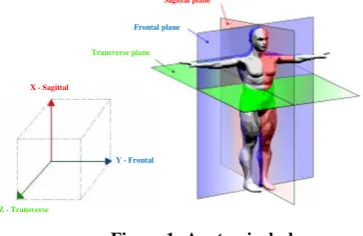
one plane is required in the same time we may use three digital cameras one for each plane. These planes are shown in Figure 1. The system is capable of analyzing the video sequence to measure the human joints movements.
Figure 1: Anatomical planes
Movements can be defined as an object's relative change of place or position in space within a time frame and with respect to some other object in space. Thus, movement may be measured by analyzing its position before and after an interval of time. While linear motion is readily demonstrated in the body as a whole as it moves in a straight line, most joint movements are combinations of translatory and angular movements that are more often parallel to the cardinal planes rather than diagonal. In addition to muscle force, joint movement is governed by factors of movement freedom, axes of movement, and range of motion. The human skeletal system is often simplified into the major joints in the body which is shown in Figure 2a. This is considered as a skeleton model which can be projected after scaling and alignment into any human position as shown in Figure 2b. This figure also shows the degrees of freedom of each of the major joints.
Figure2: a) Skeleton model, b) Skeleton projection along with the degree of freedom for major joints
Degrees of freedom (DOF) are related to the movement possibilities of rigid bodies. Kinematic definition for DOF of any system or its components would be ―the number of independent variables or coordinates required to ascertain the position of the system or its components‖. The study of joints movements is concerned with kinematics as it lets us describe the characteristics of a joint movements and position. The whole system is illustrated in Figure 3.
3.
METHODOLOGY
3.1
Video preprocessing
Before using the digital camera video sequence for later process, it should be preprocessed by smoothing in order to maximally reduce noise or instability, and then some of the frames are discarded according to a threshold function that determines the amount of movement occurred in these frames, and if it was too low these frames would be automatically discarded.
Figure 3: Main Structure of the System
3.2
Frames preprocessing
For each of the remaining frames we do the following: - Subtract the background to obtain Colored Frames for the
Whole body (CFW)
- Subtract non-moving parts of the body to obtain Colored Frames for only the Moving part in the body (CFM) - Apply Binarization to CFW to obtain Binary Frames of the
Whole body (BFW)
- Apply Binarization to CFM to obtain Binary Frames of the Moving part of the body (BFM).
3.3
Detecting and classifying the end sites
(head, limbs)
Curve Detection: By detecting curvatures contour of the
BFW. For more robustness, if we still could not find all the end sites we are looking for as they are shaded by the body, we also detect the curvature contour of the CFM to be able to detect the end site of the moving limb even after being shaded by the body. However, if we succeeded in detecting the shaded moving end site and we still could not find all the end sites, this means that there is an end site that is shaded and in the same time is not moving, so we also detect the curvature contour of the CFW in order to find it, but although this case will take more processing, it is a very rare case which rarely happen as the subject is normally instructed to make its initial position in which the limbs are fully extended along the body.
Figure 4 shows that all the end sites were successfully detected even the right arm which was shaded by the body.
1 DOF 3 DOF
3 DOF
2 DOF
2 DOF 2 DOF 3 DOF 3 DOF
a
b
Sagittal plane
Frontal plane
Transverse plane
X - Sagittal
Y - Frontal
[image:2.595.57.239.124.242.2]Head Detection: By matching the detected curvatures with a head/shoulder template contour.
Limbs Detection: By selecting high positive convex
curvatures other than the boundaries of the detected head.
Figure4: a) After detecting curvatures contour of the BFW, we could not find all the end sites since the right arm is shaded by the body, b) After detecting curvatures contour of the CFW, c) All the end sites were successfully
detected including the shaded right arm.
3.4
Calculating the body kernel
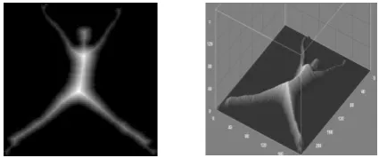
[image:3.595.54.281.114.247.2]By applying Euclidean distance transformation to both BFW and BFM then combining the two to formulate the body kernel. Figure 5 shows the result of applying distance transformation.
Figure 5: The result of applying distance transformation
3.5
Calculating the skeleton
Which is the set of connected pixels in the middle, and it is considered as the medial axis of the original body representing its topology. It can be obtained by applying erosion and thinning algorithm to the body kernel.
3.6
Classifying skeleton typical points
As shown in Figure 6- Skeleton point: Two neighbours - Branch point: Three neighbours - End point: One neighbor
Figure 6: Classifying skeleton typical points, Gray: Skeleton point, Dark gray: End point, Black: Branch
point.
3.7
Optimizing skeleton points
We need to search for the skeleton shape S that minimizes a function F, which measures how much the skeleton fits with the video sequence.
𝐹 = 𝛼𝐾 + 𝛽𝐸 + 𝛾𝐻 (1)
This function is based on three terms: the kernel term K, the end sites term E, and the harmonic term H. The idea is to project the skeleton template on the calculated skeleton after scaling and alignment, then optimize this projection by the optimization function.In order to adjust the scaling of theskeleton we used the method illustrated in [27].The alignment is simpler since wealready detectedthe end sites positions and can be calculated on the skeletonby projection [28].
However, to get the kernel term we need to select some points on the skeleton including all the template joints then calculate their average kernel values at their locations
𝐾 = − 𝑘 𝑡 (𝑝 𝑛 × 𝑇 𝑡, 𝑆 )
𝑁 𝑛
(2)
Where 𝑘 𝑡 is the kernel at time 𝑡, 𝑝 𝑛 is the nth selected point on the skeleton, 𝑇 𝑡, 𝑆 is the transform that converts the local coordinate vector of 𝑝 𝑛 to its location, and N is the total number of selected points.
However, to get the end sites term, we need to make sure that the projected locations of the end sites are near the detected end sites:
𝐸 = 𝛿 𝑚 − 𝜌(𝑚) 2
𝑀 𝑚
(3)
Where, δ(m)is the mth detected end site, ρ(m) is its corresponding projected end site, and M is the total identified end sites at the current frame.
And, to get the harmonic term, the skeleton shape should not have sudden changes over time so we compare it with other shapes from previous frames:
𝐻 = 𝑆 𝑡 − 2𝑆 𝑡 − 1 + 𝑝(𝑡 − 2) 2 (4)
After computing the three terms K, E,and H we compute the function F in equation 1 by adding them together after multiplying each term by its bias. As stated earlier our goal is to minimize F, which can cause a problem of having so many local minima. However, to overcome the problem of having so many local minima, we apply simulated annealing, to converge to the global minimum. Simulated annealing is a probabilistic method proposed for finding the global minimum of a cost function that may possess several local minima. It works by emulating the physical process whereby a solid is slowly cooled so that when eventually its structure is ―frozen‖, this happens at a minimum energy configuration. It may require only being able to evaluate the density function. This method was independently described by Scott Kirkpatrick, C. Daniel Gelatt and Mario P. Vecchi in 1983,[29] and by VladoČerný in 1985[30].It is an adaptation of the Metropolis-Hastings algorithm, a Monte Carlo method to generate sample states of a thermodynamic system, invented by M.N. Rosenbluth in a paper by N. Metropolis et al. in 1953 [31].
4.
KINEMATICS
4.1
Kinematic Modeling
Kinematics studies the motion of bodies without consideration of the forces ormoments that cause the motion. A digital human can be modeled as a mechanical system that includes link lengths and mass moments of inertia. The motion of his limbs could be approximated as an articulated motion of rigid body parts [32]-[35].
[image:3.595.61.274.359.448.2]Figure 7a depicts the modeling of a human using a series of rigid links connected by joints; the circles represent kinematic joints.
Figure 7: a) Digital human modeling using a series of rigid links connected by joints, b) Knee joint modeling using
revolute joint, c) Hip joint mechanical model
The body segments are assumed to be connected by rotational (revolute) joints. For instance, consider the right knee joint of a human, shown in Figure 7a. The knee joint is composed of ligaments and tendons between two segments, which are the femur and the tibia. Since the knee is bent in one direction, it is assumed to be a one degree of freedom revolute joint as shown in Figure 7b.
The kinematics of human locomotion describes visually observable qualities or quantities, although in many cases these can be accurately measured only by the use of instrumentation (time, distance or angles). It remains relatively stable between individuals and is obtained under the following headings: a) Temporal (Time), b) Spatial (Distance), c) Angular displacement.
A more complicated joint can be modeled in the same manner. Figure 7c depicts human hip joint anatomy and its mechanical model.
The model used in this paper, takes into account a certain revolute joints to represent each physical joint in the human. Prismatic joints, or sliding joints, could have been included, but by only including revolute joints in the human model it simplifies the skeleton, while still providing a very good approximation of gross motion for the human [36].
For instance, a ball and socket joint, like the shoulder, is modeled by three revolute joints located on top of each other and corresponds to three degrees of freedom. Examples of the joints used for the shoulder, elbow, and wrist are shown in Figure 8a.
Since the shoulder and hip joints can rotate in any direction, they are assumed to be universal joints, which have three degrees of freedom. The knee joint is assumed to be one degree of freedom rotational (revolute) joints. The elbow, wrist, and ankle joints are to be two degree of freedom rotational joints.
The joint structure of the digital human model is seen in Figure 8b; the figure shows the 53 coordinate systems and 49 DOF for the human body. The human model includes 5 chains of joints, one chain for each limb: right arm, left arm, right leg, left leg, and the head.
Figure 8: a) A human skeleton showing the physical joints and the corresponding mathematical joints and links,
b) The model for the virtual human
[image:4.595.53.281.103.213.2]In general, human locomotion means the body moves around. In other words, the global degree of freedom exists with respect to an inertial reference frame in the mathematical sense. The global degrees of freedom are composed of three translational (prismatic) joints and three rotational (revolute) joints. Figure 9 depicts how the global degrees of freedom are set up.
Figure 9: Global degree of freedom description
4.2
Kinematic Analysis
The simplest way to describe the translational and rotational relationship systematically between adjacent links in articulated chains is the matrix transformation method. The transformation matrix is represented in a 4×4 homogeneous matrix. This method represents each link coordinate system in terms of the previous link coordinate system. Any local coordinate system (including the end-effector of the manipulator or serial chain) can be expressed in a global reference frame. So, basically, the method represents a vector in one coordinate frame in terms of another coordinate frame. This method has its base in the field of robotics, but it can be used for modeling human kinematics as well.
As shown in Figure 10, any point of interest in the ith framecan be transferred to the global reference frame0r:
𝑟
0 = 𝑇
𝑖 𝑖𝑟
0 (5)
whereir is a 4×1 vector in terms of the ith reference frame and 0
Ti is a 4×4 homogeneous transformation matrix from the ith reference frame to the global reference frame. The format of the vector ir is:
𝑟𝑇
𝑖 = 𝑟𝑥 𝑟𝑦 𝑟
𝑧 1 (6)
[image:4.595.335.514.146.259.2]whererx, ry, and rz represent any point of interest in the ith frame in terms of the Cartesian coordinates.
Figure 10 Articulated chain
Here the transformation of a vector to the global reference frame is simply the multiplication of transformation matrices, which is given as:
𝑇𝑖
0 = 𝑇
1
0 1𝑇2⋯𝑖−1𝑇𝑖= 𝑇
𝑛 𝑛−1 𝑖
𝑛=1
(7)
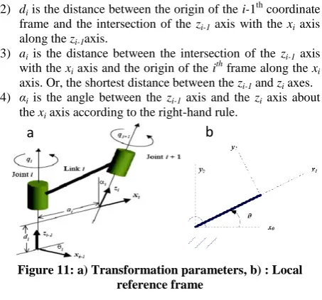
According to this method, the four parameters in Figure 11a are defined as follows:
1) θi is the joint angle between the xi-1 axis and the xi axis about the zi-1 axis according to the right-hand rule.
a
b
a
b
c
Translational joint
[image:4.595.58.265.642.730.2]2) di is the distance between the origin of the i-1th coordinate frame and the intersection of the zi-1 axis with the xi axis along the zi-1axis.
3) ai is the distance between the intersection of the zi-1 axis with the xi axis and the origin of the i
th
frame along the xi axis. Or, the shortest distance between the zi-1 and zi axes. 4) αi is the angle between the zi-1 axis and the zi axis about
[image:5.595.54.281.71.282.2]the xi axis according to the right-hand rule.
Figure 11: a) Transformation parameters, b) : Local reference frame
Then, the transformation matrix i-1Ti is composed in the following sequence of transformations:
WhereRz and Rx represent rotation about the z and x axes, respectively, and Transz and Transx represent translations along the z and x axes, respectively. In other words, Equation (8) represents the following:
1) first, the i-1th frame is rotated by angle θ about the z axis; 2) second, the rotated frame is translated by distance d along
the z axis;
3) third, the translated frame is translated again by distance a along the x axis; and
4) Fourth, the translated frame is rotated by angle α about the x axis.
This allows us to establish the home configuration, which is the starting configuration of the mechanical linkage; a suitable home configuration must be established in order to use the transformation method. In summary, to use this method, the coordinates system must satisfy the following two conditions: 1) The axis xi is perpendicular to the axis zi-1.
2) The axis xi must intersect the axis zi-1.
The transformation matrix from the ith frame to the i-1th frame is then given as:
cos 𝜃𝑖 − cos 𝛼𝑖sin 𝜃𝑖
sin 𝜃𝑖 cos 𝛼𝑖cos 𝜃𝑖 − sin 𝛼𝑖sin 𝛼𝑖sin 𝜃𝑖cos 𝜃𝑖 𝑎𝑖𝑎𝑖cos 𝜃𝑖sin 𝜃𝑖 0 sin 𝛼𝑖
0 0 0 1cos 𝛼𝑖 𝑑𝑖
(9)
In the case of a rotational joint, the joint parameters di, ai, and αi are constant (which means they are fixed). Only θi is treated as a rotational degree of freedom, qi. In a mechanical model, qi is the vector of generalized coordinates, and each transformation matrix has one degree of freedom.
The local coordinate system is located at the end of the link in this representation. So, if we consider that there is a one-degree-of-freedom manipulator as shown in Figure 11b and the global reference frame is x0, y0, z0 (z axis is perpendicular to the paper), then the local reference frame x1, y1, z1, is located at the end of the linkage, according to this method. The derivatives of transformation matrices are necessary for evaluating the equation of motion and for calculating gradients in gradient-based optimization. The derivatives are needed with respect to the joint displacements. The joint displacement that locates coordinate system i from the previous coordinate system is qi; however the displacement is added to θi for a revolute joint and di for a prismatic joint. The derivative of a single transformation matrix (i.e. between xi
and xi-1) is calculated by differentiating each entry of the matrix.
The derivative of transformation matrix from the ith frame to the i-1th frame is calculated for a revolute joint by Equation (10).
−sin 𝜃𝑖 − cos 𝛼𝑖cos 𝜃𝑖
cos 𝜃𝑖 − cos 𝛼𝑖sin 𝜃𝑖 sin 𝛼𝑖sin 𝛼𝑖cos 𝜃𝑖sin 𝜃𝑖 −𝑎𝑖𝑎𝑖cos 𝜃𝑖sin 𝜃𝑖 0 0
0 0 0 00 0
(10)
The second and third derivatives are found similarly. The derivatives of a general transformation matrix can be calculated using the chain rule. If the transformation matrix spans more than one joint, then only the transformation matrix that is a function of qi is differentiated [36], [37].
4.3
Forward and Inverse Kinematic
Human kinematics can be divided into forward kinematics and inversekinematics.In general, forward kinematics entails finding the position and orientation of a point on the body, given the angles of the joints of the body.
Alternatively, inverse kinematics entails finding the angles of the joints of the body, given the position and orientation of a point on the body or determining that there is no solution.
Forward kinematics problem is straightforward and there is nocomplexity deriving the equations. Hence, there is always a forward kinematicssolution of a manipulator. Inverse kinematics is much more complicated than forward kinematics, especially for a system like the human body, which is redundant, and involves a large number of DOFs.. The solution of the inverse kinematics problemis computationally expansive and generally takes a very long time in the realtime control of manipulators.
The forward kinematics specifies the Cartesian position and orientation of the local frame attached to the human limb relative to the base frame which is attached to the still joint (e.g. shoulder or hip joint). They are provided by multiplying a series of matrices parameterized by joint angles, so finding a solution isn’t difficult at all.
On the other hand, the inverse kinematics problem is ill-posed as infinite solutions exist due to the self-motion manifold, e.g. a self-motion surface, etc. [38]-[41]. With reasonable constraints or prior knowledge, a plausible solution can be found. However, our goal is to estimate the limb position, this is possible if some acquired angle-related data were given.
S. Kucuk and Z. Bingul [42], explained both forward and inverse kinematics for arobot, which is similar to human. They also provided solution techniques for this problem including analytical and numerical methods.
However, in order to reduce error rate as much as possible, after analyzing the video sequence and acquiring both positions and angles for each joint, we use both methods to validate the computed data.
5.
EXPERIMENTAL RESULTS
The proposed system is computer based, where the digital camera provides a video sequence, and the software allows 300 Hz sampling rate. The computer is a PC with a Pentium (R) 4/2.4GHz CPU.
The kinematic data of the human limbs of a three subjects during daily activities were collected using motion capture system at a sampling frequency of 120 Hz. The subjects were instructed to perform three repetitions of the same activity.
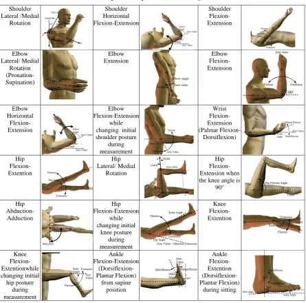
The activities were divided into two subgroups: (1) general motions, and (2) actions. Selecting the specific human activities was based on previous surveys of the disabled community indicating the desired tasks and functionality of powered orthotic devices and rehabilitation programs [43]-[46]. The general motion included a movement through a full range of motion of each of the human joints in different postures. The human actions during daily activities were performed in different body postures depending on the nature of the activity.
Given these conditions, no external forces or torques were applied on the human. Every action and general motion started from an initial position in which the limbs were fully extended along the body. The activities in Table1 were included in the experimental protocol.The movement dynamics were captured for each subject using analytical and numerical approaches. A model of the subject is then
developed and its data is stored. In addition, the dynamics of the subject body is simulated numerically using a numerical model.
[image:6.595.76.522.268.708.2]Figure 12, illustrates the movement angles after three repetitions of three activities of the hip joint along the three planes of movement (sagittal, frontal, and transverse) which are computed and displayed as a trace graph with degrees of movement plotted against time and look somewhat smooth and stable. These three activities are flexion/extension, abduction/adduction, and lateral/medial rotation of the hip joint; they are illustrated in figure 13. In the hip joint activities the flexion/extension appear on the Sagittal plane with a range of motion 0°-126° (0-2.2 RAD), abduction/adduction appear on the Frontal plane with a range of motion 0°-46° (0-0.8 RAD), and lateral/medial rotation appear on the Transverse plane with a range of motion 0°-44.5° (0-0.76 RAD).
Table 1: Activities included in the experimental protocol (first 19 are general motions, last 2 are actions).
Shoulder Lateral /Medial
Rotation
Shoulder Horizontal Flexion-Extension
Shoulder Flexion-Extension
Elbow Lateral/ Medial
Rotation (Pronation-Supination)
Elbow Extension
Elbow Flexion-Extension
Elbow Horizontal
Flexion-Extension
Elbow Flexion-Extension
while changing initial shoulder posture
during measurement
Wrist Flexion-Extension (Palmar
Flexion-Dorsiflexion)
Hip Flexion-Extention
Hip Lateral/ Medial
Rotation
Hip Flexion-Extension when the knee angle is
90°
Hip
Abduction-Adduction
Hip Flexion-Extension
while changing initial
knee posture during measurement
Knee Flexion-Extention
Knee Flexion-Extentionwhile changing initial hip posture
during measurement
Ankle Flexion-Extension
(Dorsiflexion-Plantar Flexion)
from supine position
Ankle Flexion-Extention (Dorsiflexion-Plantar Flexion)
during sitting
Abduction
Ankle Lateral/ Medial
Rotation
Shoulder Complex Motion including Flexion-Extension and
Adduction-Abduction
Hip Complex Motion
including Flexion-Extension and
Adduction-Abduction
For the purpose of validation, static ranges of movements were measured by goniometer. That is, the subject performs the required movement then holds the final position whilst the measurement of that movement is taken by the goniometer. However, dynamic movements, including combinations of movements and the velocity of movement, which can be captured by the system, cannot be captured by the goniometer and so a complete picture of the movement is not obtained. This may be particularly clear in the movement of a complex joint, like the shoulder and hip joints, where movement is three-dimensional. These goniometer measurements were compared to the system results and the average difference was less than 2% in all cases.
6.
CONCLUSIONS & FUTURE WORK
In this paper, we developed a computer vision system that is capable of analyzing and measuring human joints movements which can provide an attractive alternative to manual instruments such as goniometer, inclinometer or a tape. In addition, this system can provide an opportunity to perform accurate measurements without using expensive sensors, or special environments. Furthermore, it is easy to use, without any difficult requirements, and gives the opportunity for physiotherapist to diagnose and aid rehabilitation of joint movement disorders.Although this kind of research yields valuable information, it only takes in to consideration revolute joints to represent each physical joint in the human. However, further research on prismatic joints is needed.
7.
REFERENCES
[1] AnkurAgarwal, Bill Triggs, "Tracking articulated motion using a mixture of autoregressive models", in: Proceedings of the European Conference on Computer Vision (ECCV’04), Lecture Notes in Computer Science, vol. 3 (3024), May 2004, pp. 54–65.
[2] AnkurAgarwal, Bill Triggs, "A local basis representation for estimating human pose from cluttered images", in: Proceedings of the Asian Conference on Computer Vision (ACCV’06)—Part 1, Lecture Notes in Computer Science, vol. 3851, January 2006, pp. 50–59.
[3] AnkurAgarwal, Bill Triggs, "Recovering 3D human pose from monocular images", IEEE Transactions on Pattern Analysis and Machine Intelligence, vol. 28 no. 1, January 2006, pp. 44-58.
[4] Jake K. Aggarwal, Qin Cai, "Human motion analysis: a review, Computer Vision and Image Understanding" Vol. 73, No. 3, March 1999, pp. 428-440.
[5] Park, W., "Data-Based Human Motion Simulation", in Handbook of Digital Human Modelling, Taylor & Francis Group,LLC, 2009, p. 9.
[6] Abdel-Malek, K., and Arora, J. (2009), "Physics-Based Digital Human Modeling:Predictive Dynamics," in Handbook of Digital Human Modelling, ed. V. G. Duffy.
[7] S. Biswas, M. Quwaider, ―Body posture identification using Hidden Markov Model with wearable sensor networks‖, International Conference on Body Area Networks, March 2008, pp. 52-59.
[8] H. Y. Lau, K. Y. Tong, H. Zhu, ―Support vector machine for classification of walking condition using miniature kinematic sensors‖, Med. Biol. Eng. Comput., Vol. 46, No. 6,June 2008, pp. 563-573.
[9] H Zhou and H. Hu, ―A survey - human movement tracking and stroke rehabilitation‖, Technical Report CSM-420, ISSN1744-8050, University of Essex, 2004.
[10]Farrell, K. and Marler, R.T., 2004, "Optimization-based kinematic models for human posture", SAE Digital
Sagittal Plane
Frontal Plane
Transverse Plane Figure 13: In the hip joint activities the
flexion/extension appear on the Sagittal plane,abduction/adduction appear on the Frontal plane, and lateral/medial rotation appear on the Transverse plane
Sagittal Plane
Flexion/Extension Abduction/Adduction Lateral/Medial Rotation
Flexion/Extension Abduction/Adduction Lateral/Medial Rotation Flexion/Extension Abduction/Adduction Lateral/Medial Rotation
Frontal Plane
Transverse Plane
Actual Values Improved Values
Actual Values Improved Values
[image:7.595.55.523.68.377.2]Actual Values Improved Values
[image:7.595.56.276.479.605.2]Human Modeling for Design and Engineering (June 14-16, 2005), Iowa City, IA.
[11]Computer aided kinematics and dynamics of mechanical systems, by E. J. Haug, Allyn and Bacon, Boston, 1989.
[12]Dariu M. Gavrila, "The visual analysis of human movement: A survey", Computer Vision and Image Understanding, Vol. 73, nr. 1, 1999, pp. 82-98.
[13]Thomas B. Moeslund, Erik Granum, "A survey of computer vision-based human motion capture", Computer Vision and Image Understanding Vol. 104 No. 2, November 2006, pp. 90-126.
[14]Thomas B. Moeslund, Adrian Hilton, Volker Kru¨ger, A survey of advances in vision-based human motion capture and analysis, Computer Vision and Image Understanding, Vol. 104 No. 2, Nov. 2006, pp. 90-126.
[15]Liang Wang, Weiming Hu, Tieniu Tan, "Recent developments in human motion analysis", Pattern Recognition, Vol. 36, No. 3, 2003, pp. 585-601.
[16]Jessica J. Wang, Sameer Singh, "Video analysis of human dynamics: a survey", Real-Time Imaging,Vol. 9 No. 5, 2003, pp. 321–346.
[17]Ausejo, S., and Wang, X. (2009), "Motion Capture and Human Motion Reconstruction," in Handbook of Digital Human Modeling, ed. V. Duffy.
[18]Goussous, F., Bhatt, R., Dasgupta, S., and Abdel-Malek, K., "Model Predictive Control for Human Motion Simulation", doi:10.4271/2009-01-2306.
[19]Silva, M., Abe, Y., and Popovic, J. , "Simulation of Human Motion Data Using Short-Horizon Model Predictive Control", ACM Transactions on Graphics (TOG) - Proceedings of ACM SIGGRAPH 2008, Vol. 27 Issue 3, August 2008, Article No. 82.
[20]Cohen, M.F., ―Interactive spacetime control for animation‖, Computer Graphics, Vol. 26, No. 2, 1992.
[21]Xiang, Y., Chung, H.-J., Kim, J., Bhatt, R., Rahamatalla, S., Yang, J., Marler, T., Arora, J., and Abdel-Malek, K., "Predictive Dynamics: An Optimization-Based Novel Approach for Human Motion Simulation", Structural and Multidisciplinary Optimization, Vol.41, No.3, Aug 2009.
[22]Shao, W. and Ng-Thow-Hing, V., 2003, ―A general joint component framework for realistic articulation in human characters‖ In Proceedings of the 2003 Symposium on interactive 3D Graphics, April 27-30, 2003), New York, NY, pp. 11-18.
[23]Rahmatalla, S., Xiang, Y., Smith, R., Li, J., Meusch, J., Bhatt, R., Swan, C., Arora, J., and Abdel-Malek, K. (2008), "A Validation Protocol for Predictive Human Location," 2008 SAE International.
[24]K.D. Nguyen, I.M. Chen, Z. Luo, S.H. Yeo, H.L. Duh, ―A wearable sensing system for tracking and monitoring of functional arm movement‖, IEEE/ASME Transactions on Mechatronics, Vol. PP, No. 99, Feb. 2010, pp. 1-8.
[25]K. Lorincz, B. Chen, G. W. Challen, A. R. Chowdhury, S. Patel, P. Bonato, M. Welsh, ―Mercury: A wearable sensor network platform for high-fidelity motion analysis‖, Embedded Networked Sensor Systems Conf.(SenSys'09), 4-6 November 2009.
[26]Mark Hall, Eibe Frank, Geoffrey Holmes, Bernhard Pfahringer, Peter Reutemann, Ian H. Witten, ―The WEKA Data Mining Software: An Update; SIGKDD Explorations, Vol.11, No.1,2009, pp. 10-18.
[27]Jerome Vignola, Jean-François Lalonde and Robert Bergevin,―Progressive Human Skeleton Fitting‖. Proceedings of 16th Conference, Vision Interface, 2003.
[28]Chen, C., Zhuang, Y.T. and Xiao, J. (2006) "Towards robust 3D reconstruction of human motion from monocular video", Proceedings of ICAT, LNCS, Hangzhou, Vol. 4282, pp.594-603.
[29]Kirkpatrick, S.; Gelatt, C. D.; Vecchi, M. P. "Optimization by Simulated Annealing". Science, New Series, Vol. 220, No. 4598. (May 13, 1983), pp. 671-680.
[30]Černý, V. "Thermodynamical approach to the traveling salesman problem: An efficient simulation algorithm", Journal of Optimization Theory and Applications,1985, 45:41–51, doi:10.1007/BF00940812.
[31]Metropolis, Nicholas; Rosenbluth, Arianna W.; Rosenbluth, Marshall N.; Teller, Augusta H.; Teller, Edward, "Equation of State Calculations by Fast Computing Machines", The Journal of Chemical Physics,Vol. 21,No. 6, 1953,pp. 1087.
[32]A. Ude, ―Robust estimation of human body kinematics from video,‖ in IROS’99, 1999, pp. 1489–1494.
[33]Ayoub, M. M. and Lin, C. J., ―Biomechanics of manual material handling through simulation: Computational aspects.‖, Computers and Industrial Engineering, Vol. 29, No. 1,1995,pp. 427-431.
[34]Phillips, C.B., Zhao, J., and Badler, N., 1990, ―Interactive real-time articulated figure manipulation using multiple kinematic constraints‖, ACM SIGGRAPH Computer Graphics, Vol. 24, No. 2, pp. 245-250.
[35]Zhao, J. and Badler, N.I., 1994, ―Inverse kinematics positioning using nonlinear programming for highly articulated figures‖, ACM Trans. Graph., Vol. 13, No. 4, pp. 313-336.
[36]Emily Horn, ―Optimization-Based Dynamic Human Motion Prediction", University of Iowa, December 2005, (MS Thesis).
[37]Hyun-joon Chung,"Optimization-based dynamic prediction of 3D human running",Theses and Dissertations(2009), University of Iowa.
[38]Grochow, K., Martin, S.L., Hertzmann, A., and Popović, Z., 2004, ―Style-based inverse kinematics‖, ACM Transactions on Graphics, Vol. 23, No. 3, pp. 522-531.
[39]Mi, Z., Yang, J., and Abdel-Malek, K., 2002, "Real-time inverse kinematics for humans," Proceedings of 2002 ASME Design Engineering Technical Conferences (September 29-October 2, 2002), Montreal, Canada.
[40]Tolani, D., Goswami, A., and Badler, N., 2000, ―Real-time inverse kinematics techniques for anthropomorphic limbs‖, Graphical Models, Vol. 62, No. 5, pp. 353-388.
[42]SerdarKucuk, ZaferBingul,"Robot Kinematics: Forward and Inverse Kinematics",Industrial Robotics Theory Modelling& Control,2006, ISBN:3-86611-285-8
[43]Xiang, Y., Arora, J., and Abdel-Malek, K., "OptimizationBased Motion Prediction of Mechanical Systems: Sensitivity Analysis", Structural And Multidisciplinary Optimization, Vol.37, No. 6, 2007, pp.595-608.
[44]TanmayPawar, SubhasisChaudhuri, Siddhartha P. Duttagupta, ―Body movement activity recognition for ambulatory cardiac monitoring‖, IEEE Transactions on
Biomedical Engineering, Vol. 54, No. 5, May 2007, pp.874-882.
[45]Abdel-Malek, K., Yu, W., Jaber, M., and Duncan, J., ―Realistic Posture Prediction for Maximum Dexterity‖, SAE Transactions Journal of Passenger Cars-Mechanical Systems, Vol. 110, Section 6, 2002, pp. 2241-2249.