Swarm Optimization based Controller for Temperature Control of a Heat Exchanger

Swarm Optimization based Controller for Temperature

Control of a Heat Exchanger

S. Rajasekaran

Research Scholar Anna University of Technology

Coimbatore, India

Dr. T. Kannadasan

Professor of Chemical Engineering Coimbatore Institute of Technology

Coimbatore, India

ABSTRACT

In This paper uses an Attractive-Repulsive Particle Swarm Optimization (ARPSO) method for determining the optimal parameters of proportional-integral-derivative (PID) controller for temperature control of a shell and tube heat exchanger. Most of the heat exchange process is characteristic of nonlinear, large time delay and time varying. For such process it is very difficult to tune its controller parameters based on traditional PID tuning. The proposed method has excellent features, including high computational efficiency, quick stable convergence and easy implementation than standard PSO. In the proposed system, the ARPSO is implemented by MATLAB and compared with standard PSO and Genetic Algorithm (GA). The result shows that the proposed system has a more efficient in improving the step response characteristics such as reducing the steady state error, rise time; settling time and maximum peak overshoot in temperature control of a shell and tube heat exchanger.

Keywords

Heat exchangers, PSO, PID controller, tuning

1.

INTRODUCTION

Heat exchangers are one of the simplest and fundamental units in process industries such as gas processing and petrochemical industries. It exchanges the heat among more than one fluid with different temperatures outstanding to their higher efficiency, more compact structure and low cost. Heat exchangers performance affects the total plant operation directly. Controlling the heat exchanger system properly by the principle of automatic control and optimization theory is very important to build a plant with good performance [16]. Compared with other methods the PID controller is more effective and economical. The heat exchanger system has highly nonlinear features. When the operating point changes a little, the dynamic performance of the system may change a lot. For this reason, controller of heat exchanger needs to respond accordingly and work well under different operating process. The key of a PID controlling system is an optimal design of PID parameters. It affects the controlling effect directly.

Recently, many modern control methodologies such as nonlinear control, optimal control, variable structure control and adaptive control of shell and tube heat exchanger. However, these approaches are either complex in theoretical bases or difficult to implement. PID control with its three term functionality covering treatment to both transient and steady state response, offers the simplest and yet most efficient solutions to many real world control problems. The design of PID controller requires the value of parameters such as proportional gain (KP), integral time constant (KI) and

derivative time constant (KD). It has been a crucial problem to

tune properly the gains of PID controller because many industrial plants are often burdened with the characteristics such as higher order, time delay, and nonlinearities. Traditionally, the problem has been handled by a trial and error approach

.

Lin et al. [18] have introduced GA-based PID control for different applications. Genetic algorithm is a stochastic optimization algorithm that is originally motivated by the mechanism of natural selection and evolutionary genetics. Though the GA methods have been employed successfully to solve complex optimization problems, recent search has identified some deficiencies in GA performance. This degradation in efficiency is apparent in applications with highly ‗epistatic‘ objective functions (i.e., where the parameters being optimized are highly correlated), the crossover and mutation operations cannot ensure better fitness of offspring because chromosomes in the population have similar structure and their average fitness are high toward the end of the evolutionary process [1]. The PSO methods have been employed successfully to solve complex optimization problems. PSO first introduced by Kennedy and Eberhart [2] is one of the modern heuristic algorithms; it has been motivated by the behavior of organisms, such as fish schooling and bird flocking. Generally, PSO is characterized as a simple concept, easy to implement, and computationally efficient. Unlike the other heuristic techniques, PSO has a flexible and well-balanced mechanism to enhance the global and local exploration abilities [2], [3]

.

In this paper, a novel Attractive-Repulsive PSO-based approach [13] to optimally design a PID controller for a temperature control of a shell and tube heat exchanger system is proposed the results compared with standard PSO and GA based PID.

2.

HEAT EXCHANGER SYSTEM

2.1

Temperature control system

[image:2.595.77.234.94.243.2]

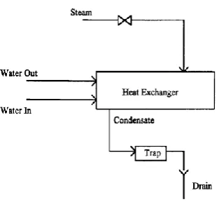
Fig 1: Shell and Tube heat exchanger

The dead-time also depends on the location and the method of installation of the temperature-measuring devices. Hence, conventional controllers based on linear systems theory can control this process only in a specific operating region for which they are tuned. To take into account the non-linearity and the dead-time, gain scheduling features and dead-time compensators have to be added. Also, the process is subjected to various external disturbances such as pressure fluctuations in the steam header, disturbances in the water line and changes in the inlet steam enthalpy and so on. The conventional controllers have to be coupled with feed forward controllers to maintain the process at its set point when disturbances occur. But, the feed forward controllers also have to be retuned for different operating conditions [15].

2.2

Dynamical Equations of Heat

Exchanger System

The heat exchanger dynamical equations can be expressed in the following term [14].

'

(

)

(

)

c c c

c T

i

T

o

UA T

c

T

o

V

c c c o

c T

 











(1)

'

(

)

(

)

h h h

c T

v

T

c

UA T

c

T

o

V

h h h o

c T

 











(2)

Ti Inlet temperature cold water, ºF T0 Outlet Temperature of cold water, ºF

Tv Inlet Temperature of hot water, ºF



Tc Outlet Temperature of hot water, ºF



c Flow rate of cold water, lb/time



h Flow rate of hot water, lb/time



i Density

Ci Specific heat

U Heat transfer co-efficient

The model equations given above are derived from first principles [17]. the objectives is that the output temperature of the cold fluid ‗T0’ to track the step input change in hot fluid inlet flow rate ‗



h‘.

3.

OVERVIEW OF PARTICLE

SWARM OPTIMIZATION AND ITS

VARIANTS

3.1

Basic Particle Optimization

Algorithm

PSO is one of the optimization techniques and a kind of evolutionary computation technique. The method has been found to be robust in solving problems featuring nonlinearity and non differentiability, multiple optima, and high dimensionality through adaptation, which is derived from the social-psychological theory [10]. The technique is derived from research on swarm such as fish schooling and bird flocking. According to the research results for a flock of birds, birds find food by flocking (not by each individual). The observation leads the assumption that every information is shared inside flocking. Moreover, according to observation of behavior of human groups, behavior of each individual (agent) is also based on behavior patterns authorized by the groups such as customs and other behavior patterns according to the experiences by each individual. The assumption is a basic concept of PSO [9]. In the PSO algorithm, instead of using evolutionary operators such as mutation and crossover, to manipulate algorithms, for a d-variabled optimization problem, a flock of particles are put into the d-dimensional search space with randomly chosen velocities and positions knowing their best values so far (Pbest) and the position in the d-dimensional space. The velocity of each particle, adjusted according to its own flying experience and the other particle‘s flying experience. For example, the

i

th particle is represented as

x

_i



(

x

_i,1

,

x

_i,2

,...

x

_{i d,}

)

in the d-dimensional space. The best previous position of

i

th _{particle is recorded and}

represented as:

Pbest_i= (Pbest_i,1, Pbest_i,2,….., Pbest_{i d,} )

The index of best particle among the entire particle in group is gbestd. The velocity for particle

i

is represented

as

v

_i



(

v

_i,1

,

v

_i,2

,...

v

_{i d,}

)

. The modified velocity and position of each particle can be calculated using the current velocity and the distance from Pbest_{i d,} to gbestd as shown in

the following formulas

( 1)

, , 1 , ,

2 ,

.

*

() *(Pbest

)

*

() *(gbest

)

t t t

i m i m i m i m

t m i m

v

w v

c

rand

x

c

Rand

x



_

_

_





(3)

, t i d

x

x

_{i m}(_,t1)



x

_{i m}t_,



v

_{i m}(_,t1)

x

_{i m}(_,t1)



x

_{i m}t_,



v

_{i m}(_,t1) (4)

i

= 1, 2…

n

m

= 1, 2…

d

Where

n

Number of particle in the group

d

Dimension

t Pointer of iteration

, t i m

min max ,

t

d i d d

V



v



V

W inertia weight factor

c c

₁

,

₂ Acceleration constant

rand

()

Random number between 0 and 1

,

t i d

x

Current position of particle i at iteration

3.2

Overview of Attractive-Repulsive

PSO Algorithm

The PSO algorithm used to solve various problems similar to applications traditionally employed in genetic algorithm and other evolutionary algorithms. So PSO has been applied to combinatorial type problems; for instance, lot sizing problem, permutation flow shop sequence problem.

The ARPSO brings a few modifications on the PSO, Riget and Vesterstrom [13] created the ARPSO to overcome the premature convergence weakness of the PSO. The attraction phase and repulsion phase are two different stages that the model is in when updating velocity of a particle. When the ARPSO in the attraction phase, it functions exactly as PSO developed by Kennedy and Eberhart. That is, the velocity update formula operator is addition. However, when the ARPSO is in the repulsion phase, the velocity update formula operator is subtraction among the velocity variables. Hence, the APRSO is an adjustment of the PSO heuristic, it has the same flexibility with the PSO yet is more effective and efficient to solve discrete or continuous optimization problems to which the PSO has been applied. Sharing many similarities with the PSO, the ARPSO algorithm begins with a random initialization of a population of individual particles in the search space once the swarm size has been quantified. According to Clerc each particle has the following features: (1) it has a position and a velocity, (2) it knows its position and the objective function value for this position, (3) it knows its neighbors, the best previous position and objective function value (variant: current position and objective function value), and (4) it remembers its best previous position. At each time cycle, the behavior of a given particle is a compromise between three possible choices: (1) to follow its own way – how much the particle trusts itself now, (2) to go towards its best previous position – how much it trusts its experience, and (3) to go towards the best neighbor‘s best previous position, or towards the best neighbor (variant) how much it trusts its neighbors [4]. Once this is completed, the global best of all particles, neighborhood best, and the local best ―thus far‖ of each particle is calculated.

1

[

1 1

(

,

)

2 2

(

,

)]

t t l t t g t t

v





wv



dir r c p



x



r c p



x

(5)

1 ,

[

,

(

1

)]

t t vi ei nb t t

x

_

 

x

insertswap

p

v

_ (6)

, , , , ,

1 1

1

( )

(

)

s N

lb i j t i j t

i j

diversity s

p

x

s L

 



 



(7)

Where

v

_t and

x

_t are velocity and position of some particle at time step t, respectively. Parameters

p

_{l t,} ,

p

_{nb t,} , and

, g t

p

are the best local position per particle, best neighbor‘s

current position per particle‘s neighborhood, and best global position in the entire swarm at time step t, respectively. The learning parameters w, c1, c2 are the cognitive and social factors which are chosen as w [0, 1] and c1, c2 [0, 2]. Variables r1 and r2 are random constants on the interval [0, 1] drawn at each time step t for each particle. Most implementations of the PSO usually have w equal to one or each particle always trusts itself. Variable dir directs the velocity of a swarm being updated by attraction ―addition (+1)‖ or repulsion ―subtraction (-1).‖ The current direction and the diversity value of the swarm greater or lower than a threshold value [17] determine if the swarm will be updated in an attraction or repulsion manner. Variable S symbolizes the swarm at discrete epochs of time. Parameter |S| and |L| represent the swarm size and the length of the longest diagonal in the search space, N is the dimensionality of the problem,

p

_{lb i j t, , ,} is the jth value of the ith best previous position per particle at time step t, and

x

_{i j t, ,} is the jth value of the ith particle at time step t.

A summary of the ARPSO algorithm for the OP as previously described is:

Parameter settings and randomize initial swarm position of particles

Initial velocity for each particle equal to zero

Initial local, global, and neighborhood, best solution of Particle exploration

Loop epoch ≤ MaxEpoch

Particle distance feasibility, shrinking, and Expansion for “

x

_t” and “

P

_{nb t,} ”

Evaluate objective function value of “

x

_t” and “

P

_{nb t,} ”

Evaluate local, global, neighborhood solution of particles explored

if ( epoch < MaxEpoch )

Attraction or repulsive direction for swarm Compute velocity “ vlbt” “ vgb,t,” and “vt”

Normalize velocity

Particle update ---swap element of

, nb t

P

into target particle

Neighborhood "

P

_{nb t,} " for each particle

4. IMPLEMENTATION

OF

PARTICLE

SWARM

OPTIMIZATION

4.1 Fitness Function

In PID controller design methods, the most common performance criteria are integrated absolute error (IAE), the integrated of time weight square error (ITSE) and integrated of squared error (ISE) that can be evaluated analytically in the frequency domain [8]. These three integral performance criteria in the frequency domain have their own advantage and disadvantages. For example, disadvantage of the IAE and ISE criteria is that its minimization can result in a response with relatively small overshoot but a long settling time because the ISE performance criterion weights all errors equally independent of time. Although the ITSE performance criterion can overcome the disadvantage of the ISE criterion, the derivation processes of the analytical formula are complex and time-consuming [17]. The IAE, ISE, and ITSE performance criterion formulas are as follows:

0 0

[( ( )

( )]

[ ( )]

IAE

r t

y t dt

e t dt

 



_





_

(8)

2 0

( )

ISE

e t dt





_

(9)

2 0

( )

ISTE

te t dt







(10)

In this paper a time domain criterion is used for evaluating the PID controller [13]. A set of good control parameters P, I and D can yield a good step response that will result in performance criteria minimization in the time domain. These performance criteria in the time domain include the overshoot, rise time, settling time, and steady-state error. Therefore, the performance criterion is defined as follows [13]:

min

_kStab

W K

( ) (1

 

e



)(

M

_P



E

_ss

)



e



(

t

_s



t

_r

)

Where K is [P, I, D], and β is the weightening factor. The performance criterion W (K) can satisfy the designer requirement using the weightening factor β value. β can set to be larger than 0.7 to reduce the overshoot and steady states error, also can set smaller than 0.7 to reduce the rise time and settling time [13]. The optimum selection of β depends on the designer‘s requirement and the characteristics of the plant under control. In this paper, due to trials, β is set to 0.5 to optimum the step response of speed control system. The fitness function is reciprocal of the performance criterion, in the other words:

1

( )

f

W K



4.2 Proposed ARPSO-PID Controller

[image:4.595.93.270.284.410.2]

The In this paper a ARPSO-PID controller used to find the optimal parameters of temperature control of a shell and tube heat exchanger. Figure 2. shows the block diagram of optimal PID control for the shell and tube heat exchanger.

Fig 2: Optimal PID control

In the proposed PSO method each particle contains three members P, I and D. It means that the search space has three dimension and particles must ‗fly‘ in a three dimensional space.

5.

RESULTS

AND

DISCUSSIONS

5.1 Optimal ARPSO-PID Response

Control the out let temperature of a shell and tube heat exchanger, according to the trials, the following ARPSO parameters are used to verify the performance of the PID-ARPSO controller parameters.

 Population size: 20;

 Wmax=0.6, Wmin= 0.1;

 C1=C2 = 1.5;

 Iteration: 20

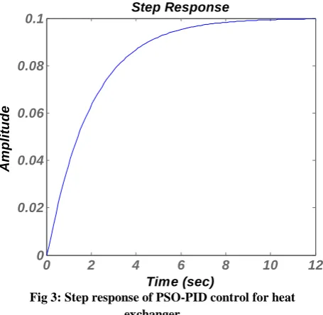
[image:4.595.321.549.522.744.2]

The response of optimal PID controller is shown in Figure 3.

Fig 3: Step response of PSO-PID control for heat exchanger

0 2 4 6 8 10 12

0 0.02 0.04 0.06 0.08

0.1 Step Response

Time (sec)

A

m

p

li

tu

d

5.2 Comparison of ARPSO-PID control

with PSO and GA control Methods

To show the effectiveness of the proposed method, a comparison is made with the designed PID controller with PSO and GA methods. At first method, the PID controller is designed using GA method [5]. Also, GA method is used to tune the PID controller. The following GA parameters which are used to verify the performance of the GA-PID controller parameters:

[image:5.595.47.264.270.456.2]

• Population size: 30 • Crossover rate: 0.9 • Mutation rate: 0.005 • Number of iterations: 30

Fig 4: Comparison between GA, LQR and PSO based PID control for heat exchanger

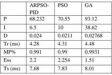
The values of designed PID Controller are 68.232, 6.5, and 0.024. Figure 4. shows the ARPSO response in comparison with PSO and GA methods and table-1 lists the performance of the two methods.

Table 1. PSO-PID, LQR and GA Performance

ARPSO-PID

PSO GA

P 68.232 70.55 93.12

I 6.5 10 38.62

D 0.024 0.0211 0.02768

Tr (ms) 4.28 4.31 4.48

MP% 0.991 0.99 0.9931

Ess 2.2 2.254 1.51

Ts (ms) 7.68 7.83 8.01

6.

CONCLUSION

This work presents an intelligent design method for the tuning problem of PID controllers for heat exchangers based on ARPSO-PID algorithm the problem of tuning PID controllers is formulated as optimization problem considering three performance indexes of transient response, the maximum overshoot, settling time and rise time. By using ARPSO-PID a solution algorithm is developed and implemented. For comparison PID controller designed by use of exiting techniques such as PSO, GA are implemented and has been shown by simulation the promising features of proposed method.

7.

REFERENCES

[1] Mitsukura.Y, Yamamoto.T, and Kaneda.M. June 1999. A design of self-tuning PID controllers using a genetic algorithm, in Proc. Amer. Contr. Conf., San Diego, CA, pp. 1361–1365.

[2] Kennedy.J and Eberhart.R. 1995. Particle swarm optimization, Proc.IEEE Int. Conf. Neural Networks, vol. IV, Perth, Australia, pp.1942–1948.

[3] Eberhart.R.C and Shi.Y. May 1998. Comparison between genetic algorithms and particle swarm optimization, Proc. IEEE Int. Conf. Evol. Comput., Anchorage, AK, pp. 11–616.

[4] Hancock.P. 1994. An Empirical Comparison of Selection Methods in Evolutionary Algorithms, Evolutionary Computing, pp.80-95.

[5] Goldberg.D and Deb.K. 1991. A Comparative Analysis of Selection Schemes used in Genetic Algorithms, Foundations of Genetic Algorithms, pp.69-93.

[6] Huang. P.Y and Chen.Y.Y. 1997. Design of PID Controller for Precision Positioning Table Using Genetic Algorithms, Proceedings of the 36th IEEE Conference on Decision and Control, pp.2513-2514.

[7] Mitsukura.Y, Yamamoto.T, and Kaneda.M. 1999. A Design of Self-Tuning PID Controllers Using a Genetic Algorithm, Proceedings of the American Control Conference, pp.1361- 1365.

[8] Clerc M, Kennedy. J. 2002. The Particle Swarm: Explosion, Stability, and Convergence in Multi-Dimension Complex Space, IEEE Transactions on Evolutionary Computation, 16(1): 58-73

[10] Sun.J, Feng.B, Xu.W.B. 2004. Particle swarm optimization with particles having quantum behavior, Proc. of 2004 Congress on Evolution Computation, Piscataway, pp.325-331.

[11] Liang.Y.C, Kulturel-Konak.S, and Smith.A.E. May 2002. Meta- heuristics for the Orienteering Problem, Proceedings of the Congress on Evolutionary Computation, Honolulu, Hawaii, pp. 384-389.

[12] Venter.G, and Sobieszczanski-Sobieski.J. 2002. Particle Swarm Optimization, American Institute of Aeronautics and Astronautics, pp. 1202-1235.

0 2 4 6 8 10 12

0 0.01 0.02 0.03 0.04 0.05 0.06 0.07 0.08 0.09 0.1

Step Response

Time (sec)

A

m

p

lit

u

d

[image:5.595.74.260.582.707.2]

[13] Riget.J and Vesterstrom.J.S. 2002. A Diversity Guided Particle Swarm Optimizer—the ARPSO, EVA-Life Technical Report.

[14] Hangos.K.M, Bokor.J, and Szederkényi.G,.2004. Analysis and control of nonlinear process control systems, Advanced Textbooks in Control and Signal Processing, 1st Edition, Ch. 4, Springer-Verlag London limited, pp. 55-61.

[15] Luyben.W.L. 1990. Process Modeling, Simulation and control for Chemical Engineers, 2nd Edition, Mc Graw-Hill Publishers.

[16] Macgregor.J.F, Wright.J, and M Hong.H. 1975.Optimal tuning of digital PID controller using dynamic stochastic models, Industrial Engineering and Chemical Process Design and Development, Vol. 14, 4, , pp. 398-402. [17] Wang.P and Kwok.D.P.1994. Optimal Design of PID

Process Controllers based on Genetic Algorithms, Control Engineers Practice, Vol. 2, 4, pp. 641-648. [18] Lin.C.L, and Jan.H.Y, and Shieh.N.C. 2003. GA-based

multiobjective PID control for a linear brushless DC motor, IEEE/ASME Trans. Mechatronics , vol.8, No. 1, pp. 56-65.