Locational planning on scenario based networks

Munich Personal RePEc Archive

Locational planning on scenario-based

networks

Photis, Yorgos N.

Department of Planning Regional Development, University of

Thessaly

5 May 1992

Online at

https://mpra.ub.uni-muenchen.de/21794/

$ .

LOCATIONAL PLANNING ON SCENARIO-BASED NETWORKS

•

Yorgos N. Photis

•

Nation al Technical University, Athens, Greece.

AbstracL More and more frequently locational planners are faced with the problem of decision making under the condition of uncertainty. In this paper a methodological framework is presented for solving Location - Allocation problems, through th e application of the multinomial logit model to data derived from t he modificati on of the characteristics of a given network. The study differs from earlier work in two aspects: First, a utility junction, as a measure of relative attractiveness, is implemented, in order to assign realization probabilities to each alternative scenari o. Second, the decisions are made through the utilizati on of two system- performance criteria. The expected loss and the minimax losscriterion of the opt imal solution of each future scenario generated by the decision maker during the problem-solving procedure of th e approach.

1.INTRODUCTION

One of t he most imp ortant issues in locational planning is t o resolve spatial problems, taking into account a set of possible alt ernatives and t heir at trib utes. Planners called to parti cipate in problem solving procedures, are more and more frequently faced wit h the problem of decision making under uncertainty . This leads to the generation, formulation and evaluation of alternative scenarios, under the assumpti on that knowledge of the costs and benefits, associated with each scenario, can help the decision maker estimate th e adoption probability of each one of them.

along any choice procedure of sufficient complexity (de Palma and Papageorgiou, 1991). Consequently, given that in locational planning the locational choices made are generally judged by th e 'quality' of the process of decision-making which generated those choices (Densham and Rushton, 1987), improved problem anal ysis will lead to better locati onal choices and thus better locati onal patterns .

We shall consider t he case when during the problem solving procedure the planner deals with a set of predefined future scenarios by a decision maker. Beginning with some init ial data and defining possible scenari os for the future , he is t rying to evaluate all feasible scenarios and their optimal soluti ons, according to their realization probability in order to improve the quality of his choices. At the beginning of the process he realizes the utility levels of each scenario. His problem then is to examine the performance of each alt ernative data set of all possible scenarios etI(UE etI), with their relative adoption probability when dealing with his location- allocation problem. In this respect, his decision will be based both on present status and the future scenarios that he imposed . In principle, all that is necessary to solve this problem is knowledge about the potential cost and benefit of each scenario rather than about the utility function of each solution. Intuitively, this process may lead to some improved locational pattern and a more robust service system . In particular, if the decision-maker adjusts only toward the future scenarios and if the above intersection has a single peak, the stationary state of his adjustment process will also maximize utility.

According to this approach, the defined scenarios by the decision maker have fixed cost and benefit attributes, assigned to them through an est imat ion rule. Hence any given scenario can arise through change combin ations of the system 's charac t eristics. Cost and benefit here and thus the altern ati ve attribute values should be understood as cardinal measures of attractiveness in terms of preference elicitation.

We imagine that the decision-maker draws a random network

to estimate with accuracy the true utility of each scenano and he is subject to framing. Since errors hav~ many causes in a randomly changing envir onment , the errors mad e during th e scenario formulation process of the approach app ear to be independent from one-another. Furthermore, since they are unpredictable, t he difference between reality and his perceptions can only be determined by a probability distribution, which serves as a "black box" to summarize complex behavioral aspects of the decision maker. Such ambiguit y is deeply rooted in the real world, and it differs from that in the literature concerned with the implications of an uncertain future on rational choice [Drese 1974).

Our paper consists of the following sections. Section two describes the model and contains its main implications .It introduces the idea of a system being in a state of change and focuses on the generation of future data sets and the estimation of scenario probabilities. Section three examines th e approach of scenario-based decision making. In our model, the relevant attractiveness of each alternative scenario is established, as has already been mentioned , via its cost and benefit definition . Section four deals with a numerical example, based on a simple network , consist ent with our framework, focusing on how the definition of alternative future scenarios affects the generation of viable alternatives for action by the decision makers . We end this paper with some brief comments, mainly about general locational analysis methodological aspects .

2. THE MODEL

In our model we use the following notation: We consider a network ~of i demand points , with which we associate a demand weight Wi ' which is a measure of

the import ance assigned to the point , and we select a list of j (j ~ i) potential sites to est ablish an activity. Fur t hermore, network data reflect the types of the network links in terms of connection quality and related range of travel times . The travel t ime between site j and point i is denoted ~j' while the associated link type is

denoted k_ij. Henceforth, d_ij will be th e adjusted distance between i and j with

(1) d.. = g..

*

The above network with its set of characteristics that interact within a context of demand and supply we will furth er on call a system and Dt will be th e complete data set associated with it . In the given network, the locations of the j facilities and the allocations of th em will be defined through the application of a location-allocation model.

In every case, when within the limits of a given system demand is covered by a set of facilities, the location of those centers is the compromise between the need for effectiveness and equity (Koutsopoulos, 1989). The modification of the values of these criteria after a time period calls for adjustments, by the decision makers, which tend to raise the system's decreasing attractiveness .

In terms of retaining a competitive position, planners and decision makers must deal with the uncertainties inherent in the problem environment . This demands, first , the generation of a set of dI(UEdI ) alternative possible future scenarios, where n;+t..t the complete network data set for time t+t..t and second ,

the design of strategies that are viable in the long run considering both the system's current status and future trends . Through the identification of the criti cal elements that give rise to uncertainty, the next step is to formulate the alternative future scenarios by considering the different possible states these elements may attain.

Ignoring exogenous factors , we consider the syst em at time t which might move to another state at time t+t..t. Unable to predict the behaviour of the decision maker with perfect certainty and if the utility measure is directly proportional to the choice probability, we treat the alteration of the system 's characte ristics as a

random phenomenon and use probabilities to describe th e alteration propensities (Figure 1). Let II'U denote the scenario probability, which is the probability that the

Figure 1. T he system.

Scenari os

Future

Today

1

-(t)

Our choice modeling from a set of mutually exclusive alternatives uses the concept of utility maximization from the field of discrete choice analysis. The prin ciple behind this is th at the decision maker is modeled as selecting the alternative with the highest utility among those available at the time the choice is made. Since the estimation and specification of a discrete choice model always successful in predicting the chosen alternatives, by all individuals should be considered impossible, we adopt the concept of random utility (Thurston, 1927). We consider t he true utilities of the alternatives random variables, so the probability tha t a specific alternative is chosen, is defined by the probability that this alterna tive has the greatest utility from the choice set , which in our case contains all alt ernatives that are known to the planner during the decision process. The type of choice set that we will focus on in this paper is where the alternatives are naturally discontinuous.

T he internal mechanisms utiliz ed by the planner in order to proceed with t he available informati on and finally arrive at a unique choice from a choice set containing two or more alternati ves is called a decision rule. In our model the decision rule will be the utility function, meaning that the attractiveness of an alternative, which is normally expressed by a vector of attribute values, is reduced to a scalar.

The most difficult assumption to make involves the form of the utility

function . In our model , we impose an additive utility function of the following

st ruct ure:

(2)

when _fl1,fl2,fl3~ 0are parameters that express the tastes of the decision maker.

3. THE SCENARIO-BASED DECISION MAKING APPROACH

3.1 R.EALIZATIOll PI.OBABILITIES OF SCEllU10S

Time is partitioned into present t and a period of length /it. At time t we have a

network configuration Dt, which is defined by the system's characteristics. On the

other hand, the planner defines the set S (UES) of scenarios for time t+/it, which

during the interval [t,t+/it] lead to a set S of future network configurations Dt+/it,

0'

where a = 1,...•s. Changes in the system characteristics through this interval are

driven by flows of change and the need for modification and adjustment.

AsSUlIPTIOll 3.1: The adoption of a specific scenario 0' for time t+/it is associated

with its relative cost and benefit CO' and B_u' and respectively with the Realization

RLS[u] of0' that has the following structure:

(3)

where fll,fl2~ 0 are the parameters that express the tastes of the decision maker with

fl1+fl2= 1 and thus

(4)

The realization utilityof the scenario 0', defined by the decision maker and

struct ure:

(5) RUTIL[,'] =

RLS[a]

+

where RLS[a] is the nonrandom systematic component; and E(fis the random error

term. We may call E

Ua scenario-specific error term becauseit can assume different

values for different scenarios.

We have already explained why the random errors are stochastically independent . If further, they are identically distributed, and if the preference ordering of the decision maker is invariant under uniform expansions of the choice set, then according to Yellot (1977, theorem 6) the random errors are double exponential . Under these circumstances, we can write the random errors as

(6) E =_I_ E r O dtor j),

>

(J J1.

where 1/j),is the dispersion parameter ofE(f' and where E is double exponential with

zero mean and unitary dispersion parameter. Then, following Mc Fadden (1974), the marginal adoption probabilities of each alternative scenario are given by the multinomiallogit model (ML, Ben-Akiva and Lerman 1985):

(7) IP(f = exp[[j],RUTIL[aJ]

(~exp

[lJ1R

l])

with

LIP

S

Since errors become smaller for larger j}" this parameter can be interpreted as the ability of the planner to estimate the true utility of a future scenario: larger j),

implies larger ability . We also have

(8) limlP = _ 1_ for U = 1,...,s

O a s

(9)

{

1 i f RUTIL[uJ = max{RUTIL[v], v = l ,...,s} limlP =

a

p,.... '" Ootherwise

That is, when there is no ability to estimate the true utility of future scenarios, alternatives are equiprobable irrespectively of differences in th eir current marginal values; and when the ability to estimate the true utility of t he future scenarios is perfect, the best estimation is made with certainty. More generally, the discriminatory power of the decision-maker is reflected on the distribution of the marginal scenario probabilities around alternatives of higher marginal utility. As the ability to estimate the utility of the alternative future scenarios increases so does the discriminatory power, and the distribution of marginal scenario probabilities, until, at the limit, the decision-maker adjusts only toward best alternatives.

3.2 SOLUTIOII EVALUATIOII CUTEUA

Let us denote L_u the optimal solution for the configuration of scenario a, if this is realized and z(b,u) the value of the objective function if solution L_b is imposed but

o is realized (b,UES). When S contains more than one scenario, the planner can solve his problem for the s alternative network configurations and then examine the performance first , of each optimal solution L;+t>t and second, the performance of

each configuration if the optimal solution of scenario b is imposed but scenario a is achieved (b,UES).

3.2.1 Expected Loss of scenario

At t he end of the problem solving procedure for every b,uES, we can const ruct a "decision matrix" [DZ

bu] whose elements will be dzbu' representing the loss in the

soluti on performance of scenario a if the optimal solution of scenario b is adopted . Consequently, if the realization probabilities of each alternative scenario are known in advan ce th en the planner may proceed with his choice through two different appr oaches. In the first one, he calculates the expected loss of each scenario E

b which is the summation of the losses dz[b,u] in the objective function if th e solution of scenario b is implemented but scenario a is realized times II'a' which is the

(10)

and

(11)

E_b =

LIP

a

-E = _{min {Eb}· IfbES}

3.2.2 Minimization of maximum loss

In the second approach, the planner searches for the solution L_b which minimizes

the maximum loss in the objective function of every other alternative scenario 0",

when b is imposed but 0" is finally achieved. In this regard

(12) zb = min{max[dz(b,O")]}

b a

Dealing with locational planning problems, both in the private and the public sector, requires the selection of the appropriate objective function (OF) which in most instances can be expressed in terms of optimization toward the fundamental objectives of the problem to be solved . We thus arrive at the optimization issue of the process and in this regard, we have defined the different data sets that will be utilized by the location-allocation model through the appropriate objective function and the allocation rule. In the next section we present a numerical example. This example, will demonstrate the generation of alternative scenarios by the decision maker and the construction, by the planner, of the decision table mentioned above.

4. A NUMERICAL EXAMPLE

In this section we consider the problem of a planner dealing with a set etf(O"Eetf) of alternative system configurations for a ten-node network :7 (i,j E.Y). In this ten-node network and concerning time t, data refer to the demand matrix W~, with

1

w·

>

L~.

K~ .,

connection types k. . ranging between 1,2 and 3. The straight distances for time t IJ

and the link types for time t, t+fl.t are displayed in Table 1. The travel time mat rix

D~. , shown in Table 1, can then be written as

IJ

(13)

[D~ ~

=

I IJ IJ

Table 1. Straight Distances for time t and Link Types for times t, t+fl.t.

From T6traight t # 1 # 2 # 3

Node Nodslstance

1 2 10 1 1 1 1

1 6 12 3 1 1 1

1 9 25 3 3 2 1

2 3 11 2 1 2 2

2 5 12 2 1 2 2

3 7 14 3 3 2 3

4 5 6 3 3 2 3

4 6 15 2 1 2 2

4 9 16 3 3 2 3

4 10 9 2 1 2 2

6 9 14 2 1 2 1

7 8 7 2 1 2 1

7 10 18 3 3 2 1

8 10 13 3 3 2 3

Table 2. Distance matrix for time t .

Node 1 2 3 4 5 6 7 8 9 10

1 10 32 52 34 36 74 88 64 70

2 22 42 24 46 64 78 74 60

3 64 46 68 42 56 96 82

4 18 30 71 57 48 18

5 48 88 75 66 36

6 101 87 28 48

7 14 119 53

8 105 39

9 66

10

On the basis of the model developed in section two and in terms of scenario

definition , the decision maker is enabled to modify both the demand W~ and the

I

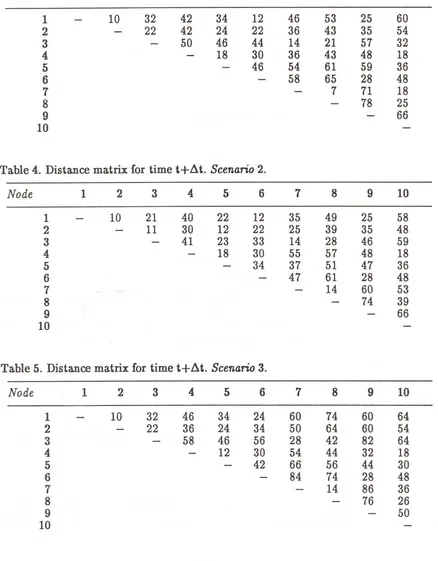
there are three alternative scenarios riI= {1,2,3} , for whi ch associated shortest-path distances and demand matrices are shown in tables 3, 4, 5 and 8.

Table 3. Distance matrix for timet+~t. Scenario 1.

Nod e 1 2 3 4 5 6 7 8 9 10

1 10 32 42 34 12 46 53 25 60

2 22 42 24 22 36 43 35 54

3 50 46 44 14 21 57 32

4 18 30 36 43 48 18

5 46 54 61 59 36

6 58 65 28 48

7 7 71 18

8 78 25

9 66

10

Table 4. Distance matrix for timet+~t . Scenario 2.

Node 1 2 3 4 5 6 7 8 9 10

1 10 21 40 22 12 35 49 25 58

2 11 30 12 22 25 39 35 48

3 41 23 33 14 28 46 59

4 18 30 55 57 48 18

5 34 37 51 47 36

6 47 61 28 48

7 14 60 53

8 74 39

9 66

10

Table 5. Distance matrix for time t+~t. Scenario 3.

Nod e 1 2 3 4 5 6 7 8 9 10

1 10 32 46 34 24 60 74 60 64

2 22 36 24 34 50 64 60 54

3 58 46 56 28 42 82 64

4 12 30 54 44 32 18

5 42 66 56 44 30

6 84 74 28 48

7 14 86 36

8 76 26

9 50

According to assumption 3.1 the adoption of a specific scenario a at time t+,c,t is associated with its relevant cost and benefit respecti vely Caand Ba where

(14a)

(14b)

In order to calculate the attributes of these variables for each scenario a,

the decision maker imposes some simple translation rules:

TUIISLATIOII lULE 4.1: The modification of the weights of the nodes from w

t at

time t to Wa at time t+,c,t, leads to a weight-specific cost C

wuand benefit Bwuof scenario a.Actually,

TUIISLATIOII lULE 4.2: The modification of the type of the connection between

nodes i and j from T

t at time t to Ta at tim e t+,c,t , leads to a

type-of-connection-specific cost C_{T u} and benefit BTu of scenario a. The smaller

the numeri cal value of the connection type the better it is and thus , the closer the travel time gets to actual distance. On this basis,

future network configurations.

Table 6. Scenario associated cost and benefit.

Scenario 1 2 3 434 358 317 966 683 407

Following equations (5), (15a), (15b), (16a), (16b) and after the

initialization of factor

Pi'

mostly interested in the anticipated cost of the alternative, the associated value of

t he Realization utility RUTIL[u] and the associated adoption probabilities Pa of

each scenario a, are calculated and shown in Table 8, while Table 7 shows the

adoption probabilities of each alternative scenario for the different values of PI in

the interval [t,t+t.t], while Figure 2 compares the graphical representations of the

adoption probabilities of the three alternative scenarios for different values of PI'

throughout the problem-solving approach.

1

2 3

, ' . 0 0

, , I

0.25 0 .50 0. 75

Valu e of Bl , 0 .00 -3

~

~

~

-,

~

- / "

/ /

./'

_/

~

i->

/

---i i i i I i I I I , , I I I I ,

o

Figure 2. Plot of II'

o 100

'"

....

....

<t

Table 8. Demand for time t and t+ l .t .

# 1

# 2

#.9

Node t 47.7% 31.6% 20.6%

1 12 100 70 12

2 24 38 70 24

3 32 32 80 32

4 12 12 12 40

5 16 16 16 40

6 28 28 28 40

7 23 80 23 40

8 22 30 50 50

9 44 44 44 44

10 61 61 61 61

In this example and in order to establish p facilities in p potential locations and supply each node from a subset of the established facilities , we consider a heuristic algorithm which solves the p-median problem (Densham, 1989). By definition, the p-median is a prototype formulation that reflects many realistic locati onal decision problems . The p-median problem minimizes total distance of demand from the closest of p centers in the system. It can be formulated in the following way:

(17) minimize z = '" '" x. . c. .

_{£. £.}

where x_ij = 1 is the demand node is allocated to facility j, 0 otherwise; and c_ij is a

metri c of interaction that can take various forms including distance, transport at ion cost, or travel time . In our case, where travel distan ce minimizati on is the objective,

(18) c.. = w· d..

Ij 1 IJ

where wi is demand weight of node i, that is the amount of demand to be served at

the it h locati on, and d_ij is the adjusted distance from the it h to the jth location,

objec t ive funct ion for th e optimal solution and th e loss in the object ive fun ct ion in

th e case we adopt th e optimal solution of scenario b, but a is achi eved for all b,aES .

Following eq uations ( 10) , (11) and (12) we fill t he Expect ed Loss and Mini max Loss

columns of th e table. The evaluation and compari son of the alternatives and t he

results in our example, shows that scenario

#

Loss and the minimum Maximum Loss for the current problem formulation .

Table 9. Solution Evalnation Table

Realized Scenario

Adopted Scenario #1 #2 #3 Expected Maximum

#1 (11'1=47 .7%) 0 4538 1404 1702 4538

#2 (11'2=31.6%) 3554 0 5406 2841 5406

#3 (11' 3= 20.7%) 1140 5862 0 2364 5862

Table 7. Scenario probabilities as a function of PI'

Alternative values ofP I

a 0.000 0.167 0.333 0.500 0.667 0.833 1.000

1 94.1% 90.5% 84.5% 75.8% 63.3% 47.7% 31.3%

2 5.5% 8.6% 13.3% 19.2% 26.0% 31.6% 33.6%

5. CONCLUDING REMARKS

Uncertainty is inherent in most locational planning situations, due to the dynamic nature of the problem environment and the inability of the planners to predict with accuracy, the exact future system configuration and network specification. Nevertheless, it is exception rather than the rule that such considerations are studied in locational decision problems. In this paper we presented a scenario-based locational planning (SBLP) framework. We deal with the problem of assigning probabilities to each alternative future scenario defined by the decision maker, through the application of the multinomial logit model. Still , by no means, we can say that we are able to localize the one and only scenario whose optimal solution is a global optimum. Nevertheless, knowing the nature of locational planning and the problems faced within the context of scenario-based location analysis, we argue, that through the implementation of our model, we can determine a more reasonable decision making process, due to the definition of the utility function as cost and benefit-oriented. Undoubtedly, there are many possible types of change in the problem environment and consequently, a plethora of ways of translating them to cost and benefit and incorporating them in the general framework . In our numerical example, we examined the case when only the weights of the nodes and the types of the connections can be modified through the scenario generation and formulation stages of the approach, .bearing in mind that, the overall objective of this paper is to provide insights about methodologies, which can contribute to the solution of locational decision problems in practice, where we believe that there is a strong need for further refinements.

decisions, being more vital than a ' realist ic' location-allocation model. As Krarup and Pruzan stated (1990):

T here is no doubt th at l ocat io na l decisi on probl ems focus upon st rategic

rather tban tactical matters, for example where to place sch ools rather than

how to route scho ol buses- That is ) the emphasis is placed upo n plan ning

and design problems rathe r than on operational prc blee s- It should b e

noted however that in practice a Ioeational decision prob l em can se ldo m be

cons idered in isolation from other strat eg ic de c is

ions-Although we deal with a rather simplified case, our approach can be

REFERENCES

Aho A V, Hopcroft J E, Ullman J D, (1983). Data structures and algorithms.

Addison-Wesley Publishing company Reading, Massachusetts .

Ben-Akiva M, Lerman S R, (1985). Discrete Choice Analysis: Theory and

Application to Travel Demand. Cambridge, Mass: MIT Press.

De Palma A, Papageorgiou Y, (1991). "A model of rational choice behaviour under imperfect ability to choose", forthcoming .

Densham P J, Rushton G, (1987). "Decision Support systems for Locational Planning", in Behavioural Modeling in Geography Eds R G Golledge and H Timmermans. Croom Helm, New York, NY

Densham P J , (1989). Computer Interactive Techniques for Settlement

Reorganization, Ph.D. Dissertation, Department of Geography, The University of Iowa.

Dreze J H, (1974). "Axiomatic Theories of Choice , Cardinal Utility, and Subjective

Probability: A Review" . In J . H. Dreze (ed .), Allocation Under

Uncertainty: Equilibrium and Optimality, Wiley, New Work, 3-23 .

Faludi A, (1973). Planning Theory. Pergamon Press, Oxford .

Ghosh A, Me Lafferty S L, (1987). Location strategies for retail and sennce

firms.Lexington books, Toronto.

Ghosh A, Rushton G, (1987) . Spatial Analysis and Location -Allocation Models.

Van Norstrand Reinhold Company, New York.

J ones J C, (1970), Design M ethods : Seeds of Human Fut ures. J ohn Wiley,

Chichester, Sussex.

Koutsopoulos K, (1989). Geography and Spatial Analysis. Papadamis, Athens ,

Gree ce.

Krarup J , Pruzan P M, (1990) . "Ingredients of Locati on Anal ysis", in Discrete Location Theory Eds P B Mirchandani and R L Francis, Wiley , New York. Lolonis P , (1990). "Methodologies for supporting Locati on Decision Making : State of

the art and research directions" Discussion paper 44, Department of Geography, The University of Iowa, Iowa City, Iowa.

Love R F , Morris J G, W esolowski G 0, (1988). Facilit ies location: Models &

Liaw K-L, (1990), "Joint Effects of Personal Factors and Ecological Variables on the Interprovincial Migration Pattern of Young Adults in Canada: A Nested Logit Analysis." Geographical Analysis 22, 189-208 .

March J G , (1978). "Bounded Rationality, Ambiguity and the Engineering of Choice". Bell Journal of Economics 9,587-608.

McFadden D, (1974). "Conditional Logit Analysis of Qualitative Choice Behaviour". In P. Zarembka (ed.), Frontiers in Econometrics, Academic Press, New York, 105-142.

Mirchandani P B, Francis R L, (eds.), (1990). Discrete location theory. Wiley Interscience, Chichester, Sussex.

Von Neumann J, Morgenstern 0, (1947). Theory of Games and Economic Behaviour. Princeton University Press, Princeton, NJ.

Reggiani A, Stefani S, (1986). "Aggregation in decisionmaking: a unifying approach". Environment and Planning A 18, 1115-1125.

Roszak T, (1987). The Cult of Information and the True Art of Thinking.

Lutterworth Press , Cambridge.

Samet H, (1990) . The Design and Analysis of Spatial Data Structures. Addison Wesley , Reading MA.

Thomas M J, (1979). "The procedural planning theory of A Faludi'', Planning Outlook22 (2) 72-77.

Thurston L, (1927). "A Law of Comparative Judgement" . Psychological Review 34,

273-286 .

Weisbord Parcelli Kern ,(1984)