Government Institute for
Economic Research
Working
Papers
55
Taxable Income Elasticity and the Anatomy of
Behavioral Response: Evidence from Finland
VATT WORKING PAPERS
55
Taxable Income Elasticity and the
Anatomy of Behavioral Response:
Evidence from Finland
Tuomas Matikka
Many thanks to Jarkko Harju, Markus Jäntti, Jani-Petri Laamanen, Seppo Kari,
Tuomas Kosonen, Kaisa Kotakorpi, Teemu Lyytikäinen, Jukka Pirttilä, Marja
Riihelä, Friedrich Schneider, Håkan Selin, Jeffrey Smith, Roope Uusitalo and
Trine E. Vattø for their useful comments and discussion. I also thank the
participants at many conferences and seminars for their helpful comments. All
remaining errors are my own. Funding from the Academy of Finland, the Finnish
Cultural Foundation, the Nordic Tax Research Council, the Emil Aaltonen
Foundation and the OP-Pohjola Group Research Foundation is gratefully
acknowledged.
Government Institute for Economic Research, tuomas.matikka@vatt.fi
ISBN 978-952-274-108-0 (PDF)
ISSN 1798-0291 (PDF)
Valtion taloudellinen tutkimuskeskus
Government Institute for Economic Research
Arkadiankatu 7, 00100 Helsinki, Finland
Edita Prima Oy
Helsinki, February 2014
Taxable Income Elasticity and the Anatomy of Behavioral
Response: Evidence from Finland
Government Institute for Economic Research
VATT Working Papers 55/2014
Tuomas Matikka
Abstract
This paper uses extensive Finnish panel data from 1995–2007 to analyze the
elasticity of taxable income (ETI). I use individual changes in flat municipal
income tax rates as an instrument for the overall changes in marginal tax rates.
This instrument is not a function of individual income, which is the basis for an
exogenous instrument in the taxable income model. In general, instruments used
in previous studies do not have this feature. Furthermore, I estimate behavioral
responses using smaller subcomponents of taxable income, such as working
hours, fringe benefits and tax deductions. This “anatomy” of overall ETI has
rarely been studied in the literature. The results show that the average ETI
estimate in Finland is 0.35–0.60, depending on the empirical specification and
the degree of regional controlling. Subcomponent analysis suggests that neither
work effort nor labor supply respond actively to tax changes. In contrast, it seems
that fringe benefits and deductions from taxable income might have a larger
effect.
A new version of this paper has been published in VATT Working Paper series:
The Elasticity of Taxable Income: Evidence from Changes in Municipal Income
Tax Rates in Finland, VATT Working Papers 69, 18.12.2015.
Key words: Personal income taxation, Elasticity of taxable income, Deadweight
loss
JEL classification numbers: H21, H24, H31
Tiivistelmä
Tässä tutkimuksessa tarkastellaan verotettavan tulon joustoa (Elasticity of
taxable income) Suomessa vuosina 1995–2007. Verotettavan tulon jousto on
keskeinen tekijä verotuksen taloudellisen tehokkuuden ja veronmuutosten
vaikutusten arvioinnissa. Verotettavan tulon jousto mittaa sitä, kuinka paljon
tuloverotuksen veropohja eli verotettava tulo keskimäärin muuttuu, kun yhdestä
lisäeurosta käteen jäävä osuus (1-rajaveroaste) muuttuu yhden prosentin.
Verotettavan tulon jousto mittaa kattavasti tuloverotuksen aiheuttamaa
hyvinvointitappiota. Eri tavat reagoida tuloverotukseen vaikuttavat kaikki sen
taloudelliseen tehokkuuteen (Feldstein (1999)). Korkeampi rajaveroaste voi
esimerkiksi vähentää tehtyjä työtunteja sekä lisätä verosuunnittelua ja
verovähennysten käyttöä. Verotettavan tulon jousto huomioi eri kanavat joilla
tuloverotukseen voidaan reagoida. Verotettavan tulon jouston lisäksi tässä
tutkimuksessa tarkastellaan laajan rekisteriaineiston avulla sitä, mistä tekijöistä
verotettavan tulon jousto Suomessa koostuu. Tutkimuksessa hyödynnetään
kunnallisveroprosenteissa tapahtuneita henkilötason muutoksia veroastevaihtelun
lähteenä. Kunnallisverotus tarjoaa hyvän vertailuasetelman, sillä
kunnallisveroprosentit ovat muuttuneet eri tavalla eri puolella Suomea eri
vuosina. Lisäksi kunnallisveroprosentti ei riipu henkilön tuloista, joten
kunnallisveroprosentin muutokset aiheuttavat muutoksia rajaveroasteissa yli
tulojakauman. Tulosten perusteella verotettavan tulon jousto on Suomessa
keskimäärin 0.35. Tulosta voidaan tulkita siten, että tuloverotuksen kiristäminen
(keventäminen) pienentää (kasvattaa) verotettavaa tuloa tilastollisesti
merkitsevällä tavalla, mutta tuloverotuksen aiheuttama hyvinvointitappio on
kokonaisuudessaan maltillinen. Tutkimustulokset antavat lisäksi viitteitä siitä,
että työtunnit ja tuntipalkka eivät reagoi herkästi rajaveroasteen muutoksiin. Sen
sijaan vaikuttaa siltä, että epäsäännöllisemmät tulot kuten luontoisedut sekä
verovähennysten määrä, selittävät huomattavan osan verotettavan tulon joustosta.
Tästä tutkimuksesta on julkaistu uusi versio: The Elasticity of Taxable Income:
Evidence from Changes in Municipal Income Tax Rates in Finland, VATT
Working Papers 69, 18.12.2015.
Asiasanat: Tuloverotus, verotettavan tulon jousto, hyvinvointitappio
JEL-luokitus: H21, H24, H31
Contents
1 Introduction 1
2 Conceptual framework 4
2.1 Taxable income model . . . 4
2.2 The marginal excess burden of income taxation and the components of taxable income . . . 5
2.3 Empirical model . . . 7
2.4 Components of total taxable income . . . 9
3 Finnish income tax system and recent tax reforms 10 3.1 Institutional setting . . . 10
3.2 Recent changes in income tax rates . . . 11
4 Data and identification 13 4.1 Data . . . 13
4.2 Individual tax rate variation . . . 14
4.3 Net-of-tax rate instrument . . . 17
4.4 Descriptive statistics . . . 19
4.5 Estimable equation . . . 22
5 Results 23 5.1 Taxable income elasticity . . . 23
5.2 Subcomponents of taxable income . . . 25
5.3 Alternative specifications and sensitivity checks . . . 27
1
Introduction
The elasticity of taxable income (ETI) with respect to the net-of-tax rate (one minus the marginal tax rate) is a key tax policy parameter and an important element in the efficiency analysis of income taxation. The practical significance of ETI is straightfor-ward: it measures how a one percent change in the net-of-tax rate affects taxable income. Intuitively, the more elastic taxable income is, the larger the behavioral response to a tax reform will be, in terms of a change in the tax base. From the efficiency point of view, a large ETI makes a tax increase relatively costly and a tax decrease less costly, and vice versa. Under general conditions, ETI has been shown to measure the marginal deadweight loss of income taxation (Feldstein (1995, 1999)). In addition to labor supply responses, ETI also covers changes in, for example, effort and productivity, deduction behavior, tax evasion and tax avoidance. All of these margins are (more or less) impor-tant when considering the overall efficiency of a tax system. Altogether, good knowledge of country-specific ETI is essential when deciding on national tax reforms.
Earlier empirical literature has focused on estimating the overall elasticity of taxable income. It is still largely unknown which of the behavioral margins are the most respon-sive components of the total elasticity. However, detailed knowledge of “the anatomy of behavioral response” (Slemrod (1996)) could also be useful when designing an income tax system and the detailed structure of tax reforms, especially in the light of minimizing the excess burden of income taxation.1
Furthermore, analysis of different subcomponents provides information on the actual economic nature of the response. It is rather difficult for the policymaker to influence deep individual utility arguments, such as the opportunity cost of working. However, for example, it is easier to influence tax deduction behavior even through minor adjustments to regulations. In addition to overall ETI, the rich register-based panel data I use in this study enables me to approximate the net-of-tax rate elasticities of the subcomponents of total taxable income, such as labor supply and deduction behavior.
The source of individual variation in tax rates and the endogeneity of the net-of-tax rate variable are the main issues to focus on when estimating ETI using panel data. Identification requires variation in income tax rates that is different for individuals with otherwise similar income trends. Also, due to the progressive income tax rate schedule, a valid instrument for the net-of-tax rate is usually necessary in order to derive a consistent elasticity estimator. In this study I use variation in municipal-level flat income tax rates for both purposes.
1In previous studies, Blomquist and Selin (2010) estimate the elasticity of the hourly wage rate. Using
a Swedish data set, they find a significant wage rate response. Also, Kleven and Schultz (2013) report that capital income components of taxable income are more responsive than earned income in Denmark. Previous literature concerning tax reforms in the United States shows that a large proportion of the behavioral response of high-income individuals has been in the form of tax avoidance via income-shifting rather than real economic behavior (see for example Slemrod (1995, 1996), Gordon and Slemrod (2000), Goolsbee (2000), Saez (2004), and Saez, Slemrod and Giertz (2012))
Finnish municipal taxation has appealing features from the point of view of empirical ETI analysis. Firstly, the municipal income tax rate is proportional, which means that it is independent of individual income level. This is the basis for using changes in municipal tax rates as an instrument for changes in overall individual net-of-tax rates in the empirical ETI model. Recent literature highlights that frequently used predicted net-of-tax rate instruments are not necessarily consistent (see for example Blomquist and Selin (2010)). These instruments are functions of individual income in the base period, and thus possibly endogenous in a model where changes in taxable income are regressed with changes in the instrumented net-of-tax rate.
Another key feature of the variation in municipal tax rates is that different municipalities have changed their tax rates differently in different years. In other words, net-of-tax rates have changed differently for otherwise similar individuals who differ only in location. Moreover, as the municipal income tax rate does not depend on individual income, changes in municipal taxation have an effect on net-of-tax rates throughout the income distribution. This makes it possible to identify the average elasticity parameter while avoiding some of the usual difficulties in ETI estimation, namely non-tax-related changes in the shape of the income distribution and the mean reversion of income. These issues are particularly troublesome if tax rate variation is concentrated in a single part of the income distribution, such as in the case of tax reforms affecting only high income earners. Many earlier studies base their estimation strategy on tax rate variation that occurs only at a certain income level.
However, changes in municipal income tax rates are not randomly assigned. Munici-palities might change their tax rates based on, for example, previous trends in average taxable income in their jurisdiction. This might affect the validity of the instrument. As a potential solution, the data include a variety of municipal characteristics that I use to control for municipal-level economic circumstances. In addition, I apply different combinations of year and regional fixed effects in the estimable equation, and study the effect of previous income trends on future tax changes in order to assess the exogeneity of the instrument.
To sum up, this study contributes to the empirical ETI literature in three ways: first, I use a net-of-tax rate instrument that is uncorrelated with individual income level. This enables the exogeneity of the instrument. Secondly, the differential tax rate variation used in this study covers the entire income distribution. This improves the identification of the average ETI, which is the parameter of main interest in this study. Also, the data I use include a variety of socio-economic variables such as age, marital status, education, gender, the size of the household and information on various social benefit programs. These enable rich controlling for both permanent and transitory elements of individual income. Third, I divide the behavioral effect of tax changes into smaller components. This subcomponent analysis provides information on what the most important behavioral margins are. Studying the structure of the elasticity also shows how much of the response
is driven by changes in baseline real-term behavior (e.g. hours of work and work effort), and how much is accounted for by other margins (tax deductions, fringe benefits etc.). I estimate the average intensive margin ETI in Finland to be 0.35-0.60, depending on the empirical specification and the degree of regional and municipal-level controlling. As in many earlier studies, the average ETI is larger for women than for men, and larger for high and low-income individuals than for middle-income earners. Analysis of the subcomponents of taxable income gives tentative evidence that both work effort and labor supply are not very responsive to tax rate changes. However, more irregular components such as fringe benefits and tax deductions seem to be more responsive. These imply that a large proportion of the overall ETI is not due to changes in labor supply behavior.
The empirical ETI literature has grown substantially following the pioneering studies by Feldstein (1995, 1999). Feldstein (1995) uses panel data to analyze behavioral re-sponses to the 1986 tax reform in the US. He estimates ETI to be large, ranging from 1-3, depending on the specification used. Many studies following Feldstein (1995) fo-cus on improving the elasticity estimation by paying more attention to net-of-tax rate instruments and non-tax-related changes in the income distribution. Along with these modifications, the elasticity estimates decreased markedly compared to those in Feldstein (1995). A wide range of studies report elasticity estimates ranging from 0 to 0.6. For example, the widely cited Gruber and Saez (2002) study reports the elasticity of taxable income to be 0.18 for mid-income earners and 0.57 for high-income earners in the US. An extensive review of earlier empirical results from the US can be found in Saez, Slemrod and Giertz (2012).
More recent papers further study the reliability and consistency of the estimation of ETI by utilizing different tax reforms and different net-of-tax rate instruments. This litera-ture underlines that different tax reforms and more consistent estimation strategies do not necessarily yield estimates of a similar magnitude as in the seminal contribution of Gruber and Saez (2002). In particular, it has been shown that predicted net-of-tax rate instruments built on base-year income are not consistent due to potential endogeneity problems (see Blomquist and Selin (2010) and Weber (2013)). Many of the frequently cited studies, including Gruber and Saez (2002), build their estimators on these instru-ments.
A majority of earlier empirical studies estimate ETI using US data sets, while studies concerning European countries and other regions are less common. Particularly, there are practically no earlier Finnish ETI studies available to this day.2 For other Nordic
countries, Blomquist and Selin (2010) estimate ETI to be around 0.20 for males and 1 for females in Sweden. In addition, they document positive elasticity estimates for the hourly wage rate, and also find statistically significant income effects. For Denmark,
2Pirttilä and Uusitalo (2005) calculate approximate elasticity estimates for Finland. Their results
Kleven and Schultz (2013) use an extensive panel data and many tax reforms to analyze ETI. In general, they obtain modest elasticity estimates, the upper bound of ETI being 0.3. Also, Chetty et al. (2011) report small elasticity estimates using Danish data. For Norway, Aarbu and Thoresen (2001) find only small responses to tax changes. Using a similar approach as Auten and Carroll (1999), they report that ETI is not significantly different from zero. In a more recent paper, Thoresen and Vattø (2013) report elasticities below 0.1 for Norway.
The rest of the paper is organized as follows: Section 2 presents the conceptual framework including the theoretical background and the empirical model. Section 3 describes the Finnish income tax system and recent changes in income taxation. Section 4 introduces the data and discusses identification issues. Section 5 presents the results and Section 6 concludes.
2
Conceptual framework
2.1 Taxable income model
The basic idea of the static taxable income model is that an individual receives positive utility from consumption c and negative utility from creating and reporting taxable incomeT I.3 Following the model of Gruber and Saez (2002), the utility functionu(c, T I)
is maximized under the budget constraint c=T I(1−τ) +R, where(1−τ) is the net-of-tax rate on a linear segment of the tax rate schedule, andR denotes virtual income. Maximization of the utility function with respect to the budget constraint gives supply functions of taxable income of the formT I =T I((1−τ), R). Next, consider a marginal decrease in (1−τ) (i.e. a marginal increase in τ). The decreased net-of-tax rate will have two effects: the uncompensated substitution effect which decreases the supply of taxable income, and a compensating income effect. Taking total differentials of the taxable income supply function and using the definitions of the substitution and income elasticities, we can write the change in taxable income as
dT I T I =−ε C dτ (1−τ) +η dR−T Idτ T I(1−τ) (1)
From now on I assume that there are no income effects, i.e. η = 0. Earlier literature shows that income effects are either insignificant or very small (see Saez, Slemrod and
3Within this study, taxable income is regarded as taxable earned income. Taxable earned income is
defined as the sum of labor income and taxable non-labor income minus deductions (verotettava tulo). The legal distinction between earned income and capital income in the Finnish income tax system is described in the next section.
Giertz (2012)).4 Thus in the empirical analysis, ETI is measured by regressing changes
in taxable income with changes in the tax rate.
Some recent studies (e.g. Chetty (2012), Chetty et al. (2011), Kleven and Schultz (2013)) underline that optimization frictions have an effect on the estimated taxable income elas-ticity. In short, the theory of optimization frictions concludes that there are costs related to responding to tax changes (adjustment costs, job search costs, paying attention to tax code, filing deductions etc.), and these costs might attenuate the observed elasticities and make them less than the structural elasticities derived in a frictionless benchmark case. Obviously, frictions are more relevant when changes in the tax schedule are small. Small tax rate changes might induce only small utility benefits from changing behavior, and this utility gain might be smaller than the associated (fixed) costs. Thus small changes in tax rates tend to lead to smaller changes in observed behavior (on average).
Differential tax rate variation has been rather small in Finland over the last 20 years, at least when compared to many other countries. Therefore, assuming that adjustment costs or other frictions matter, we would expect to get smaller ETI estimates in this study. This line of thought also implies that elasticities derived using small changes in tax rates represent only the lower bound of the structural long-term tax responsiveness. However, if adjustment costs decrease over time, we would expect larger estimates when longer time horizons are studied.
2.2 The marginal excess burden of income taxation and the
compo-nents of taxable income
As shown in Feldstein (1999), all behavioral responses reflect the inefficiency of the tax system. The marginal deadweight loss of income taxation can be expressed in terms of the elasticity of taxable income and the relevant income tax rate even when individuals make various decisions in response to income taxation, such as hours of work, work effort, deduction behavior, education choices and so on. This result holds when agents do not make optimization errors and income taxation or taxable income do not impose any externalities.
Following Chetty (2009), consider an individual who makes a vector of decisions{x1, .., xn}
that all affect total taxable income linearly, additively and separately. In this framework, overall taxable income can be presented as the sum of all behavioral choices, Σxi =T I.
Assume further that each choice xi has a convex and increasing cost function gi(xi).
Each individual maximizes a quasi-linear utility function of the form u(c,Σxi) = c−
Σgi(xi)with respect toc= Σxi(1−τ) +R, wherecis consumption, R is virtual income
4However, Blomquist and Selin (2010) report statistically significant income effects in their study
using Swedish data. Nevertheless, in their study the inclusion of the virtual income term has a negligible effect on the parameter of interest, the compensated elasticity of taxable income
and τ is the common marginal tax rate for each subcomponent of taxable income. As before, I assume no income effects.
I follow the standard approach in the deadweight loss literature and compare the marginal excess burden caused by responses to a tax rate change to a benchmark case without any behavioral responses. The social welfare function W used for this purpose is presented as the sum of individual utility (in the curly brackets) and government tax revenue
W =n(1−τ)Xxi+R−
X
gi(xi)
o
+τXxi (2)
Next, consider a small tax increase dτ. As the individual has optimized his/her bundle ofxi, we can write the marginal excess burden of income taxation in the following form5
DW L= dW dτ =τ n X i=1 dxi dτ =τ dT I dτ (3)
Most of the earlier studies focus on estimating the overall average elasticity of taxable income. As underlined in Feldstein (1999), the substitution elasticities for different choices contributing toT I are not needed in order to analyze the marginal deadweight loss of income taxation, as long as individuals behave such that g′
i(xi) = τ for all i.
However, I argue that knowledge of dxi/dτ is useful when designing the income tax
system and future tax reforms. As pointed out in Blomquist and Selin (2010) and Saez (2003), this information would be valuable if we assume that taxable income itself is directly controlled by the government, which is in fact the case in practical tax policy. The endogenous choice of the tax base is analyzed more thoroughly in Slemrod and Kopczuk (2002) and Kopczuk (2005).
Analysis of the subcomponents of taxable income is more relevant when the assumption of the common income tax rate τ is relaxed. In the extreme case, when different tax rates are applied to all different xi, equation (3) can be expressed as
DW L= n X i=1 τi dxi dτi (4) where τi represents the tax rate for each xi.
Abstracting from administrative costs and putting aside tax evasion and tax avoidance, there is no explicit reason to be restricted to a single income tax rate τi = τ for all of
5Assuming that the individual makes optimal choices for eachx
iand that there are no externalities
implies thatg′
i(xi) =τfor alli(Chetty 2009). Thus, based on the envelope theorem, there are no
second-order effects on the individual’s utility. Originally, the main idea of Chetty (2009) is to show that with weaker assumptions the marginal excess burden is a weighted sum of the total earnings elasticity and the taxable income elasticity. This result holds when the marginal social cost does not equal the tax rate
for somexi. As highlighted in Chetty (2009), this might be the case in the presence of tax avoidance
with transfer costs. Specific theoretical or empirical analysis of this type of framework is, however, out of the scope of this paper.
the components of taxable income. Following the assumptions presented so far, in order to minimize the deadweight loss, tax increases should be targeted at choices that are less responsive. On the other hand, the largest economic effects can be achieved when changing the tax rate on the xi associated with the largest elasticities. In addition to
overall ETI estimates, the responsiveness of different types of subcomponents comprising taxable income are in this case the parameters of interest when designing an effective income tax system.
In addition to this Ramsey-type welfare motivation6, analysis of the anatomy of taxable
income elasticity sheds more light on the actual economic nature of the behavioral re-sponse. Distinguishing between, for example, real income creation and tax avoidance has important implications for the evaluation of an income tax system (see Slemrod (1995, 1996)). Real responses such as hours of work and work effort reflect deep individual util-ity parameters, whereas tax avoidance and tax evasion signal an ineffective and poorly designed tax system. Estimating real and “non-real” subcomponents separately helps to distinguish between the importance of the two in the sense of the marginal excess burden of income taxation.7
Finally, a thorough analysis of different subcomponents of taxable income would perhaps call for separate theoretical and empirical frameworks for all of them. However, for the sake of clarity and comparability, I abstract from separate modeling of the different components and approximate them in a single ETI framework, both theoretically and in the empirical model.8
2.3 Empirical model
This section briefly describes the general empirical methodology of estimating ETI using tax reforms and individual-level panel data.9 In short, the idea is to measure how the
net-of-tax rate affects the taxable income of an individual. Econometrically, this relationship can be described as
ln(T I)t,i=βln(1−τ)t,i+ln(µ)t,i+ln(λ)i+ln(δ)t+ln(ε)t,i (5)
whereidenotes the index for individual andtfor time. T I is taxable income and(1−τ)
is the net-of-tax rate. µt,i denotes other time-variant individual characteristics that
6In short, the well known Ramsey rule (Ramsey (1927)) suggests that goods should be taxed in
inverse proportion to their elasticities of demand.
7As emphasized in many recent US studies (see for example Gordon and Slemrod (2000), Goolsbee
(2000), Saez (2004) and Saez et al. (2012)), a large proportion of the response to recent income tax reforms at the top of the income distribution seems to be due to income-shifting or re-timing of reported income.
8For example, see Blomquist and Selin (2010) for methodological details of the wage rate estimation.
9For a comprehensive discussion of ETI estimation, including cross-sectional approaches, see Saez et
al. (2012). See Saez (2010) and Chetty et al. (2011) for a discussion on identifying ETI locally using the distribution of taxable income and the kink points in the marginal income tax rate schedule.
affect the income level differently at different times, andλi is a matrix of time-invariant
individual characteristics. δt is the general time trend and εt,i is the individual error
term, including the transitory income component.
In practice, it is difficult to identify the average effect of the net-of-tax rate on taxable income (parameter β) using equation (5). Innate ability and many other time-invariant individual characteristics are unobserved, and at the same time are correlated with the progressive tax rateτ. Therefore, in the presence of an income tax reform, one practical approach is to use a first-differences estimator of the form
ln(T I)t+k,i−ln(T I)t,i =αt+e(ln(1−τ)t+k,i−ln(1−τ)t,i)+
(ln(µ)t+k,i−ln(µ)t,i) + (ln(ε)t+k,i−ln(εt,i))
(6)
where e is the average elasticity of taxable income. In equation (6), time-invariant individual characteristics are canceled out by definition.
There are many issues that need to be considered before we can achieve a reliable estimate of ETI using equation (6). These are widely discussed in the empirical ETI literature. First, the net-of-tax rate is still endogenous. There is a mechanical correlation between
(ln(1−τ)t+k,i−ln(1−τ)t,,i)and (ln(ε)t+k,i−ln(ε)t,i) due to the progressive nature of
the tax rate schedule (i.e. higher taxable income is taxed at higher marginal tax rates). Also, a positive income shock in yearttends to be followed by lower income in the next period t+k, and vice versa. This so-called mean reversion of income combined with the progressive tax rate schedule might bias the elasticity estimate. Secondly, non-tax-related changes in the shape of the income distribution need to be taken into account. In particular, if differential variation in tax rates is concentrated only in a certain part of the income distribution, differential income growth trends in different parts of the distribution must be carefully controlled for.
Endogeneity of the net-of-tax rate can be corrected by using instrumental variable esti-mators. This obviously requires a valid instrumental variable. Non-tax-related changes inµt,i are usually controlled for by adding variants of lagged taxable income and other
individual-level controls to the model. Rich individual panel data sets might also allow for controlling the transitory elements of income (see for example Kleven and Schultz (2013)). I discuss all of these issues in more detail in Section 4.
To recap, a usual estimable equation for ETI when using individual-level panel data is of the following form:
△ln(T I)t,i =α0+e△ln(1−τ)t,i+α1ln(B)t,i+△ln(ε)t,i (7)
where △denotes the difference in the variables between t+kand t, and (1−τ) is the instrumented net-of-tax rate. In this study, I apply the changes in proportional municipal tax rates as instruments. Bt,i is a matrix of individual base-year control variables. Here
the base-year controls include income controls. One common approach is to use taxable income spline variables for richer income controlling (see Gruber and Saez (2002)).
2.4 Components of total taxable income
In addition to overall taxable income, I also estimate the elasticities of various behavioral choices{x1, ..., xn}that comprise the overall elasticity of taxable income. The estimable
behavioral margins include overall wages, monthly wage rates, fringe benefits, monthly working hours and two specific tax deductions, namely a commuting deduction and a work-related expense deduction. The data on all margins are register-based. A more detailed description of the components is presented in Table 5 in the Appendix.
The wage rate measures work effort in a broad sense. Separate analysis of fringe benefits examines whether possible effort responses are driven by irregular and non-monetary components of wages rather than regular cash payments.10 As a comparison, I also
estimate the traditional labor supply response in the form of working hours elasticity. This estimate together with the wage rate elasticity sheds light on the extent of real economy responses to income tax rate changes.
The analysis of tax deductions partly reveals the responsiveness of tax planning. A decrease in the net-of-tax rate increases the gains received from decreasing taxable in-come, and thus increases the incentives to file more deductions than before. Both of the deductions examined in this study are not automatically accounted for in individual tax-ation. In other words, in order to be eligible for the commuting or expense deductions, a taxpayer needs to fill a tax form and substantiate the desired amount of the deduction. The list of subcomponents included in the analysis is not exhaustive. This means that I cannot fully construct the total elasticity of taxable income with the (weighted) sum of all the margins estimated in this study. Furthermore, register-based data on hours and wage rates might not be fully reliable, and non-random measurement errors probably occur. Thus the analysis of the subcomponents is only intended for approximating what the most relevant parts of the behavioral response are in the sense of marginal excess burden. In general, similar econometric requirements for the net-of-tax rate variation and the net-of-tax rate instrument also apply to all behavioral margins. Therefore, municipal net-of-tax rate instruments are also used in the subcomponent analysis.
10Fringe benefit responses can also be considered a type of tax avoidance activity. For example,
taxable benefits from the use of a company car are in many cases below the actual opportunity cost of having and driving one’s own car. However, the relative advantage of fringe benefits is very case-specific in the Finnish tax system.
3
Finnish income tax system and recent tax reforms
3.1 Institutional setting
In this study I focus on analyzing the behavioral effects of changes in earned income taxation that occurred between 1995-2007. In the main analysis I focus on studying the elasticity of taxable earned income. In Finland, earned income is taxed according to a progressive tax rate schedule.11 In general, the Finnish income tax system follows the principle of individual taxation. The income of a spouse or other family member does not affect the tax rate of an individual. However, some tax deductions and received social security depend on the total income of the household.
In Finland there are three levels of earned income taxation: central government (or state-level) income taxes, municipal income taxes and mandatory social security contributions. All taxes and social security payments are administered centrally by the Finnish Tax Administration.
The central government income tax rate schedule is progressive. The nominal central government income tax rate varies from 0 to 32 per cent12, depending on (taxable) income. Social security contributions are proportional. Social security contributions include, for example, mandatory pension contributions and unemployment insurance payments. The average rate of social security contributions is around 5 per cent. Social security contributions are deductible from taxable income. Table 7 in the Appendix presents the schedule for employee social security contributions in 1995-2007.
Municipal income tax rates are flat. The average nominal municipal tax rate is 18.45 per cent. All regular income earners are subject to municipal income taxation, with the exception of individuals with very low earned income who are exempt from all taxes. There are currently 320 municipalities in Finland (in 2013).13 Municipalities have au-tonomous authority to levy income tax. Municipal council elections are held in every four years at the same time throughout the country, and each democratically elected municipal council decides and announces the municipal income tax rate on an annual basis.
There are certain legislative duties and public services each municipality has to offer and fulfill. These include, for example, public health care and social services. These commitments are partly financed by municipal income taxation.14
11Since 1993, Finland has applied the principle of Nordic-type dual income taxation, where earned
income (wages, fringe benefits, pensions etc.) and capital income (interest income, capital gains, div-idends from listed corporations etc.) are taxed separately. The capital income tax rate is flat. As is typical in a dual income tax system, the top marginal tax rate on earned income (54%) is much higher than the flat tax rate on capital income (28%). Harju and Matikka (2013) present an ETI analysis of capital income and dividend taxation of Finnish business owners.
12All tax rates presented in this Section are from 2007 if not stated otherwise.
13Figure 5 in the Appendix presents a map of Finnish municipalities and counties in 2007.
The structure and framework of municipal income taxation, including the flatness of the tax rate and the tax deductions and allowances, are regulated at the central government level. Apart from the need for a certain amount of municipal tax revenue for legislative duties and the limitations to alter the frame rules of municipal taxation, municipalities can set their income tax rates freely. As a demonstration of this argument, there is a 5 percentage-point difference between the highest (21%) and lowest (16%) municipal income tax rate in the data.
3.2 Recent changes in income tax rates
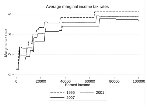
Central government income taxation From the mid-1990s onwards, there has been a general decline in central government income tax rates in Finland. Central government tax rates have decreased almost every year in all income classes more or less similarly. Figure 1 illustrates the changes in average marginal tax rates between the years 1995, 2001 and 2007. These marginal tax rates are calculated with the average municipal income tax rate in the year in question. Table 6 in the Appendix presents the marginal tax rate schedule of central government income taxation in 1995-2007.
0 .2 .4 .6 M a rg in a l ta x ra te 0 20000 40000 60000 80000 100000 Earned income 1995 2001 2007
Average marginal income tax rates
Figure 1: Average marginal tax rates in 1995, 2001 and 2007 (calculated with the average municipal tax rate in the year in question)
From the point of view of identification in the empirical ETI model, variation of this
through local tax-sharing and grants from central government. These are not directly related to the municipal tax rate in the municipality in question. For example, the degree of tax-sharing depends on the industrial and demographic structure of the municipality. Within certain limits, municipalities can also charge usage fees for statutory public services and assign low real estate taxes. In addition, part of the corporate tax revenue collected by central government is assigned to municipalities.
sort is not ideal. Although there have been significant changes in central government marginal tax rates, the generally declining nature of tax rates does not provide much differential marginal tax rate variation.
Municipal income taxation Compared to central government income taxation, changes in municipal income tax rates have been different in nature. In Finland, municipal tax rates have changed differently in different municipalities in different years.
Table 1 below presents the descriptive statistics of municipal-level tax rate changes in each year. Depending on the year, 10-30 per cent of all municipalities have changed their tax rates. On average, every fifth municipality has changed its tax rate in each year. In all of the years in 1995-2007, at least one municipality has decreased its tax rate and one has increased it.
Municipal-level tax rate changes vary from -1 to +1.5 percentage points. The average absolute change is approximately 0.5 percentage points. In general, municipal tax rates increased within the time period of 1995-2007. The average municipal income tax rate increased from 17.5% in 1995 to 18.45% in 2007.
There have also been a number of mergers (or consolidations) of two or more neighboring municipalities. Within a merger, the merged municipalities form a new municipality and decide on a new municipal tax rate. As a consequence of mergers, the total number of municipalities decreased from 455 to 416 in 1995-2007. A more detailed discussion on using the individual-level municipal income tax rate variation in the empirical analysis is deferred until Section 4.2.
Year Mean absolute change in municipal tax rate (%points) Std. Dev. Min change (% points) Max change (% points) Percent of munic-ipalities with a change in tax rate Average municipal income tax rate 1995 0.4125 0.16554 - 1 0.5 8.9 17.53 1996 0.4954 0.21983 -1 1 12.0 17.51 1997 0.5573 0.20672 - 1 1 21.2 17.42 1998 0.5478 0.22496 - 0.5 1 21.9 17.53 1999 0.5581 0.24177 - 1 1 21.9 17.60 2000 0.5326 0.20822 - 1 1 10.3 17.65 2001 0.5647 0.2194 - 0.5 1.5 25.0 17.67 2002 0.5511 0.2004 - 0.5 1 20.8 17.78 2003 0.4811 0.15387 - 0.25 1 11.9 18.04 2004 0.5533 0.2073 - 0.25 1 31.4 18.12 2005 0.5858 0.21700 - 0.5 1 31.1 18.29 2006 0.5758 0.26601 - 0.5 1.5 27.0 18.39 2007 - - - 18.45 Overall 0.5484 0.22010 - 1 1.5 18.7 17.84
Table 1: Municipal income tax rate changes ((t+ 1)−t), 1995-2007
4
Data and identification
4.1 Data
The data set I use is an individual-level panel from 1995-2007, provided by Statistics Finland. The data set consists of approximately 550,000 observations per year, which covers roughly 10% of the Finnish population.15 The data contains a wide variety of individual-level variables from different statistics. The variables are register-based. The main statistics used in this study are the personal tax record information provided by the Finnish Tax Administration, the Structure of Earnings statistics collected by Statistics Finland and municipal-level background statistics.
The data set contains all the necessary information to study the elasticity of taxable income, plus a substantial amount of individual and municipal-level control variables. Moreover, the data allow for estimating the tax elasticity of more narrow margins, such as the elasticity of working hours and wage rates based on the Structure of Earnings statistics. Table 9 in the Appendix presents the summary statistics of the key variables used in this study for individuals between 25-60 years of age. Table 9 also includes the descriptive statistics for the key municipal-level variables.
15In Finland, this register-based data set is sometimes unofficially referred to as the Jäntti-Pirttilä
4.2 Individual tax rate variation
One of the key issues in identifying the elasticity of taxable income is the source of vari-ation in net-of-tax rates. In short, differential varivari-ation in net-of-tax rates for otherwise similar individuals is needed when estimating ETI using reduced-form methods and in-dividual panel data. This study uses changes in municipal income tax rates as the main source of this variation. In the Finnish context, changes in municipal income tax rates are the main source of tax rate variation, as central government income tax rates have decreased rather similarly in all income classes.16
Compared to many of the earlier ETI studies, municipal tax rate variation has some very appealing features. First, municipal tax rate changes occur in all of the years in the data (1995-2007). There are also both increases and decreases in municipal tax rates in all of the years.
Importantly, changes in municipal tax rates affect individuals throughout the income distribution. Thus, in all income classes there are some individuals whose municipal income tax rate has changed, and some individuals faced no changes in municipal income taxation. This alleviates the potential problems associated with non-tax-related changes in the income distribution, which are critical in many earlier studies. If the shape of the income distribution varies independently of tax reforms, the analysis of behavioral responses to tax changes might give inaccurate results if this variation cannot be properly taken into account.17 As changes in municipal income tax rates are not concentrated in a certain income class or classes in any of the years, non-tax-related changes in the income distribution do not bias the elasticity estimates (at least after including appropriate covariates in the model). If nothing else, this bias is certainly much smaller than in many of the earlier studies. Furthermore, tax rate variation across the whole income distribution identifies the parameter of main interest in this study, the average elasticity of taxable income.
Figure 2 presents the actual individual marginal income tax rates at different income levels, highlighting the regional variation in marginal income tax rates. As can be seen from this figure, individuals with the same level of income face different marginal tax rates depending on the municipality of residence. Moreover, with regard to identification, individuals with the same income level face differentchanges in overall marginal tax rates due to differential changes in municipal tax rates over time.
16To my knowledge, Pirttilä and Uusitalo (2005) first proposed the use of municipal income tax rate
changes as a source of differential income tax rate variation in Finland.
17In Finland, the overall income distribution polarized between 1995-2007 (see Riihelä, Sullström and
Suoniemi (2008)). However, changes in the distribution are mostly driven by changes in capital income, not by changes in earned income, which I focus on in this study. Changes in the income distribution are also relatively modest compared to, for example, the US in the 1980s.
Figure 2: Actual marginal tax rates in 2007, including individual municipal income tax rates Year Mean absolute change in municipal tax rate (%points) Std. Dev. min change of munic. tax rate (% points) max change of munic. tax rate (% points) Percent of indi-viduals with a change in municipal tax rate 1995 0.533 0.3314 -3.25 3.75 9.6 1996 0.508 0.2504 -3.25 3.5 22.2 1997 0.632 0.2724 -3 2.75 24.2 1998 0.601 0.2888 -3 3.5 20.4 1999 0.564 0.3065 -3.25 3.75 17.5 2000 0.608 0.3411 -3.75 3.5 11.7 2001 0.605 0.2912 -3.25 3.25 23.4 2002 0.716 0.3007 -3 3.5 30.6 2003 0.581 0.2428 -2.75 3.0 17.7 2004 0.634 0.2464 -3.5 3.25 29.7 2005 0.596 0.2597 -3.5 3 22.2 2006 0.599 .03160 -4.25 3.75 15.2 Overall 0.608 0.2880 -4.25 3.75 18.7
Table 2: Individual-level tax rate variation((t+ 1)−t), 1995-2007
Table 2 describes the individual variation in municipal income tax rates. Table 2 includes individuals who faced a change in their municipal tax rate as a result of a change in their municipality of residence, or as a consequence of consolidation of two or more neighboring
municipalities.18 In the data set, 3.3% of individuals changed their municipality of
residence between t and t+ 1 (on average). This number does not include mergers of municipalities.
As can be seen from Table 2, approximately every fifth individual experienced a change in his/her municipal income tax rate each year. On average, the absolute change in the municipal tax rate was 0.6 percentage points for those individuals who faced a change in their municipal tax rate. There is a more distinctive difference between the smallest negative (-4.25 percentage points) and largest positive (3.75 percentage points) change in the municipal tax rate. The largest absolute changes are caused by changes in the municipality of residence, or as a consequence of mergers of municipalities.
Individual changes in municipal income tax rates are not very large in size. The majority of changes are between +/- 0.25-1 percentage points. When the whole net-of-tax rate is accounted for (municipal taxes + central government taxes + social security contribu-tions), most of the changes are around +/- 1-10 as a percentage. The largest changes in municipal tax rates correspond to changes in overall net-of-tax rates of +/- 5-15%. As noted in the theoretical section, very small net-of-tax rate changes might not trigger a behavioral response because the utility gain from changing individual behavior might be small on average (Chetty (2012)). In particular, the presence of large optimization frictions might attenuate the observed elasticity estimates below the underlying struc-tural long-term response.19 This is a valid point in this setup, as the variation in overall net-of-tax rates is relatively small, at least when compared to many earlier studies. On the other hand, small tax rate changes have high policy relevance. Usually income tax reforms are not particularly large. Most of the recent reforms in industrialized countries can be regarded more or less as fine-tuning of the tax systems. Therefore, a careful study of smaller-scale tax reforms might have greater practical relevance than analysis of more extensive and unique reforms, such as the tax rate cut of 1986 in the US.
In addition, it might be that the short-run response to a small change in the net-of-tax rate differs significantly from the longer-run effect, especially in the case of adjustment or search costs. Adjustment to a new level of income tax rate might easily take more than 1-3 years, particularly if the short-run gains from the behavioral response are relatively small. In the empirical part, I also test the effect of changing the time horizon in the elasticity estimate.20
Finally, as highlighted by Kopczuk (2005), changes in the tax base and the definition of
18I discuss the implications of individuals changing their municipality of residence in the next
subsec-tion.
19Using Danish data, Chetty et al. (2011) and Kleven and Schultz (2013) show evidence that the
observed elasticity estimate depends positively on the size of the change in the net-of-tax rate.
20However, as noted in Gruber and Saez (2002), theoretical prediction of the effect of the time window
on the elasticity estimate is not clear. It might also be the case that individuals react to tax changes actively in the short run, and then return to their original level of taxable income in the longer run (see for example Goolsbee (2000)). Gruber and Saez (2002) find no significant time horizon effects in their study. In contrast, Giertz (2010) reports that elasticity tends to increase as the time horizon increases.
taxable income probably affect the ETI estimate. In Finland, the definition of taxable earned income has remained relatively constant between 1995-2007. Furthermore, the minor changes in the tax base are, at least to some extent, unrelated to the main source of differential tax rate variation. This is due to the fact that the tax base and basic rules of municipal income taxation, including tax deductions and allowances, are regulated at the central government level.
4.3 Net-of-tax rate instrument
In a progressive income tax rate schedule, the marginal income tax rate increases as taxable income increases. Therefore, a change in taxable income endogenously defines the change in the net-of-tax rate. Thus the elasticity coefficient in equation (6) is very unlikely to capture the actual behavioral response to a tax rate change without using an instrumental variable estimator, and therefore a valid instrumental variable for (1−τ)
is required.
A common strategy in the earlier literature has been to simulate predicted or synthetic net-of-tax rates, and use them as instruments for the actual net-of-tax rate changes (see for example Gruber and Saez (2002)). The basic structure of a predicted net-of-tax rate variable is the following: take base year t income and use it to predict the net-of-tax rates fort+kby using the post-reform tax legislation int+k. The synthetic net-of-tax rate instrument is then the difference between the actual net-of-tax rate in t and the net-of-tax rate calculated with income in t and the tax law for t+k. The intuition behind this strategy is that the predicted difference describes the exogenous change in tax liability caused by changes in tax legislation, while ignoring any behavioral effects by keeping taxable income constant.
However, the predicted net-of-tax rate variable is a function of individual taxable income in year t. As discussed in recent ETI literature, there is no proof that this instrument is exogenous in the empirical model. Following Blomquist and Selin (2010) and Moffit and Wilhelm (2000), it is unlikely that the predicted net-of-tax rate instrument is correlated similarly with bothεt+k,i andεt,i in equation (7), as taxable income in yeartdefines the
marginal tax rate in bothtandt+k. In addition, there is no general proof that the usually added controls, mainly base-year taxable income and other individual characteristics, correct this endogeneity problem, as discussed in Weber (2013). All in all, there is concern about the validity of instruments that are explicit functions of the dependent variable.21
21Blomquist and Selin (2010) introduce a strategy where taxable income and other individual
char-acteristics at the middle year of the difference (i.e. (t+t+k)/2) are used to derive the instrument.
The middle year characteristics are used to define imputed taxable income for both tandt+k (from
which the net-of-tax rate instrument is then calculated). Blomquist and Selin (2010) show that this strategy produces exogenous instruments under relatively general assumptions about the autoregressive structure of the transitory income component. However, the validity of this type of predicted net-of-tax
In this study I use an instrument for the net-of-tax rate changes which is not a function of taxable income, namely changes in proportional municipal income tax rates. As the municipal income tax rate is flat, the tax rate is the same in all income classes within each municipality. In other words, at the individual level, the only determinant of the municipal income tax rate is the municipality of residence.22
Compared to previous studies, I do not have to make assumptions about the time struc-ture of the individual transitory income component in order to ensure the exogeneity of the instrument. In addition, as municipal income tax rates affect the net-of-tax rates in all income classes, I do not have to explicitly control for the non-tax-related changes in the income distribution in order to guarantee the causality of the behavioral param-eter. Furthermore, mean reversion does not pose a serious problem when deriving the average elasticity estimate, as yearly fluctuation in individual income does not affect the instrument.
Even though the municipal tax rate instrument is not a direct function of the dependent variable in any period, there are concerns that the instrument is not exogenous as such. The main reason for this is the possible policy endogeneity of municipal tax rate changes. In other words, municipal tax rate changes are probably not randomly assigned in the population.
In order to alleviate potential policy endogeneity, the data enable me to include vari-ous municipal-level covariates to the model, such as municipal-level unemployment and employment rates, net migration and the level of net debt. All of these variables have a presumable effect on total taxable income within a municipality, as well as average individual taxable income. For example, municipalities might increase tax rates when future tax revenue losses are predicted. This can be caused by decreased employment in the jurisdiction. Because low employment might also decrease individual taxable in-come (on average), the elasticity estimate may be upward-biased. By including a set of municipal-level covariates and other regional controls in the model, I can, at least to a reasonable extent, separate the possible municipal-level effects from the individual-level behavioral responses.
Another cause for concern is the possibility that individuals select into the “treatment” by changing their municipality of residence. First, we might worry that individuals consistently move to municipalities with lower (or higher) tax rates. However, with regard to identification in the ETI model, this is not very relevant in itself.23
attenuates whenk is large.
22The earned income tax allowance in municipal taxation depends (inversely) on earned income. This
mainly affects low-income individuals. The effect of the allowance on the effective overall net-of-tax rate is trivial for taxable income over 14,000 euros. An income cut-off of 20,000 euros is used in the estimations. The earned income tax allowance in municipal taxation is described in detail in Table 8 in the Appendix. More details on the income cut-off and other sample restrictions are provided in the next subsection.
23For example, if an individual moves to a municipality with a lower tax rate but does not change
A more serious concern would be that changes in taxable income are systematically correlated with the moving decision, and especially with the municipal tax rate in the destination municipality (i.e. the tax rate instrument is correlated with the transitory income component). For example, a new, better paid job might be a good reason for moving to another city or area. At the same time, it could be that municipalities or areas with a lot of open highly paid vacancies have a relatively low or high municipal tax rate, which would cause bias in the elasticity estimate. This is a relevant concern in the Finnish case, as the municipal income tax rates are below the average in high-wage regions such as the capital city area (Helsinki-Espoo-Vantaa). Therefore, in the baseline empirical specification, I drop individuals who change their municipality of residence betweentandt+kin order to avoid any mechanical correlation between the instrument and the transitory income component.24
4.4 Descriptive statistics
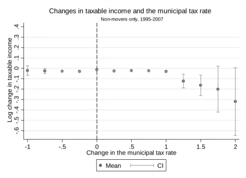
Figure 3 describes the connection between changes in individual taxable income and changes in municipal tax rates. In the Figure, I calculate and plot mean changes in log taxable income by different changes in the municipal tax rate between t+ 1 and t. Plotting mean changes in taxable income by changes in municipal tax rates is feasible as changes in municipal tax rates occur in 0.25 percentage point intervals (0.25, 0.5, 0.75 etc.). For example, the point on the dash-line in the Figure denotes the average log change in taxable income betweent+ 1andtfor those individuals who faced no changes in their municipal tax rate in the same time period.
be zero by definition even though the total taxes paid are now lower than before. Thus, this kind of purely tax-motivated migration is not an issue in this framework. Also, we might suspect that there is a classical selection problem in equation (5). The conceivable selection bias comes from the possibility that individuals who prefer low income taxation choose to reside in a municipality with a low tax rate. This preference for low income taxation is likely to be positively correlated with taxable income, causing the elasticity estimate to be biased. However, as the empirical model in question is identified by individual changes in both municipal tax rates and taxable income, this is not a very serious concern in this setup.
24In order to test the effect of moving individuals, I also estimate the model with the movers included.
In this case, I add an individual moving dummy to the estimable equation, along with the interaction terms of the moving dummy and the destination county. This controls for the average effect of moving to a certain region on individual income (given other individual characteristics).
-. 6 -. 5 -. 4 -. 3 -. 2 -. 1 0 .1 .2 .3 .4 L o g c h a n g e i n t a x a b le i n c o m e -1 -.5 0 .5 1 1.5 2
Change in the municipal tax rate
Mean CI
Non-movers only, 1995-2007
Changes in taxable income and the municipal tax rate
Notes: The baseline sample includes observations where base-year taxable income is above 20,000 euros. Pen-sioners, disabled persons and people under the age of 24 and over the age of 60 are not included in the sample. Also, the sample is limited to individuals whose absolute change in log taxable income between tand t+ 1is below 8.5, and whose marital status is unchanged between the two years. For more details, see Section 4.5.
Figure 3: Changes in taxable income and changes in municipal tax rates
From Figure 3 we can see that relative changes in taxable income are, on average, more negative the larger the positive changes in municipal tax rates are. In other words, positive changes in municipal tax rates induce negative changes in taxable income on av-erage. This reduced-form type description suggests that individuals respond to incentives created by changes in municipal tax rates.
-. 6 -. 5 -. 4 -. 3 -. 2 -. 1 0 .1 .2 .3 .4 L o g c h a n g e i n t a x a b le i n c o m e -1 -.5 0 .5 1 1.5 2
Future change in the municipal tax rate (t+1)
Mean CI
Non-movers only, 1995-2007
Changes in taxable income and future change in the municipal tax rate
Notes: The baseline sample includes observations where base-year taxable income is above 20,000 euros. Pen-sioners, disabled persons and people under the age of 24 and over the age of 60 are not included in the sample. Also, the sample is limited to individuals whose absolute change in log taxable income between tand t+ 1is below 8.5, and whose marital status is unchanged between the two years. For more details, see Section 4.5.
Figure 4: Changes in taxable income and future changes in municipal tax rates Figure 4 shows the mean changes in log taxable income with respect to future changes in the municipal tax rate (i.e. changes in the municipal tax rate between t+ 2 and
t+ 1) . Intuitively, if municipalities respond to a decrease in taxable income in the past by increasing the municipal tax rate in the future, we should see that future tax increases are more common when there is a decreasing trend in average taxable income (and vice versa). Figure 4 does not support this policy endogeneity channel. There is no statistical difference between the changes in taxable income with respect to future changes in municipal tax rates, which suggests that future tax changes are not a (direct) function of past changes in individual taxable income. However, in order to more carefully analyze possible policy endogeneity, I add municipal-level covariates in the estimable equation in some specifications.
Figures 3 and 4 include the baseline estimation sample where individuals who change their municipality of residence between t and t+ 1 are dropped out.25 Figure 6 in the
Appendix shows a similar picture for the sample including the movers. The range of changes in municipal tax rates is naturally wider when movers are included. The Figure including the movers delivers similar conclusions as before. The left-hand side of Figure 6 shows that tax increases lead to a negative change in mean taxable income, and vice versa. Also, from the right-hand side of Figure 6 we can see that endogeneity based on
25The sample includes individuals whose municipality of residence changed due to a merger of
past changes in average taxable income is not the driving force behind the results.
4.5 Estimable equation
Following Gruber and Saez (2002), I estimate different variations of the following equa-tion using a two-stage least squares estimator (tsls)
△ln(T I)t,i=α0+e△ln(1−τ)t,i+α1f(lnT I)t,i+
α2Bt,i+α3Mt,m+
X
j
α4jY EARj +△εt,i (8)
In equation (8),△ln(T I)t,i is the change in taxable income betweentandt+k(taxable
income in municipal taxation26) for individual i. △ln(1−τ)t,i is the change in the
net-of-tax rate instrumented with the change in the municipal net-net-of-tax rate. Thus e is the coefficient of interest, the average elasticity of taxable income with respect to the net-of-tax rate.
Despite the fact that in this setup the non-tax-related changes in the income distribution and mean reversion are not as problematic as in many earlier studies, I add a ten-piece base-year taxable income spline variable (denoted by f(lnT I)t,i) into the model
in some specifications. This income control serves as a proxy for individual unobserved heterogeneity in income growth, which is correlated with the time trend (Blomquist and Selin (2010)).
Bt,iis a matrix of other base-year individual control variables. Base-year variables control
for observed individual heterogeneity affecting changes in taxable income. Bt,i includes
age, age squared, county of residence, sex, level of education (highest degree), marital status27, size of the household and dummy variables indicating whether the individual has
received any taxable social security benefits28 in the base year. I also include interaction terms of sex and other controls in the model (age, education, household size and marital status). Importantly, I also add county-year fixed effects, which control for different income trends in different parts of the country at different times.
To control for the possible policy endogeneity of the net-of-tax rate instrument, I add municipal-level (m) characteristics Mt,m to the estimable equation in some
specifica-tions. Mt,m includes base-year values of municipal-level employment, unemployment,
net migration and net loan positions. These variables reflect the actual publicly avail-able information that the decision-making bodies in each municipality have on the local economy. Finally, I add year dummies to control for time.
26In Finland, the tax bases in municipal and central government earned income taxation differ slightly.
Changing the tax base to the central government income tax base does not change the results in any significant way.
27The marital status dummies include married couples, unmarried couples, singles, divorced singles
and widows/widowers.
I limit the analysis to observations where base-year taxable income is above 20,000 euros. First, the income cut-off is needed in order to eliminate any notable effect of the municipal earned income tax allowance on the net-of-tax rate instrument. Secondly, the focus of this analysis is on the intensive margin behavioral responses, which emphasizes the need for an income cut-off. Many of the social security benefits in Finland (e.g. unemployment benefits and sickness benefits) are regarded as taxable income, which creates relatively low but positive taxable income also for individuals fully or partly outside the labor force. In addition, I drop pensioners, disabled persons and people under the age of 24 and over the age of 60 out of the sample. Also, the analysis is limited to individuals whose absolute change in log taxable income betweentandt+kis below 8.5, and whose marital status is unchanged between the two years. Finally, in the baseline analysis, I drop individuals who change their municipality of residence between
t and t+k. However, the sample includes individuals whose municipality of residence changed due to a municipality merger.29
The baseline time horizon used is three years, which is customary in the literature. In order to be able to separate this middle-term elasticity from the shorter-run effects, I drop all the observations where the individual municipal income tax rate also changed betweent+ 1andt+ 2, ort+ 2andt+ 3. Finally, as a sensitivity check, one and five-year difference models are also estimated along with other alternative specifications.
Equation (8) is also used to estimate the subcomponents of overall taxable income. The subcomponents include overall wage income, monthly wage rates, taxable fringe benefits, hours of work and two particular itemized tax deductions (commuting cost and work-related expense allowances). The same set of controls and sample limitations are also applied in the estimation of these margins.
5
Results
5.1 Taxable income elasticity
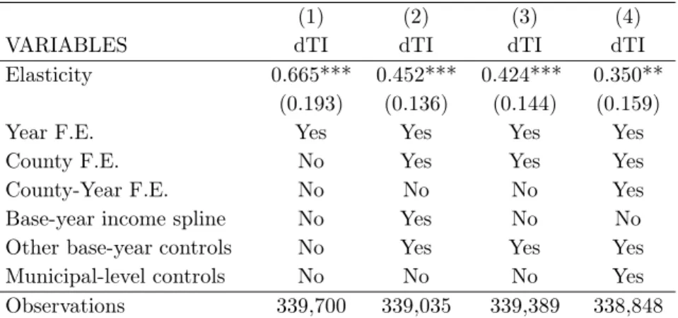
Table 3 offers the results for the three-year difference model with different specifica-tions.30
29As a sensitivity check, I also estimate the model with movers included. For the models including
the movers, Bt,i also contains a dummy variable denoting whether an individual has changed his/her
municipality of residence betweentandt+k, and the interaction terms of the moving dummy and the
county of residence int+k.
30The F-statistics for the first stage of the tsls routine are large (>100) and highly significant in
all specifications. The first-stage result for the baseline specification is presented in Table 10 in the Appendix.
(1) (2) (3) (4)
VARIABLES dTI dTI dTI dTI
Elasticity 0.665*** 0.452*** 0.424*** 0.350**
(0.193) (0.136) (0.144) (0.159)
Year F.E. Yes Yes Yes Yes
County F.E. No Yes Yes Yes
County-Year F.E. No No No Yes
Base-year income spline No Yes No No
Other base-year controls No Yes Yes Yes
Municipal-level controls No No No Yes
Observations 339,700 339,035 339,389 338,848
Robust and municipal-level clustered standard errors in parentheses. *** p<0.01, ** p<0.05, * p<0.1
Table 3: ETI estimates
First, column (1) shows the ETI estimate with only year fixed effects included in the regression. This estimate is approximately 0.66 and statistically significant at the 1% level.31 Adding controls in columns (2)-(4) decreases the point estimate. In column (2), the ETI estimate is 0.45 and statistically significant when the 10-piece base-year income spline variable and individual base-year controls are included.
In column (3) I do not include the individual base-year income spline in the equation. Without income splines the estimate is very close to that with the splines included (0.42). Firstly, this implies that income controlling does not have much effect on the ETI estimate in this particular case in which the net-of-tax rate instrument is unrelated to individual income. This can also be seen as tentative evidence that non-tax-related changes in the income distribution do not affect the elasticity estimates when tax rate variation occurs at all income levels. Secondly, base-year income is not an exogenous variable in the first-differences setup, and thus not an optimal choice as a control variable. Therefore, there are no explicit reasons why these variables need to be added to the ETI model in this case, and thus I prefer a specification in which income splines are not included.
Column (4) in Table 3 shows the preferred empirical specification with extensive regional controlling. Firstly, I add the interactions of county and year fixed effects to control for different income trends in different years in different regions. Furthermore, I add base-year municipal-level variables to the equation. As mentioned before, there might be reasons to suspect that municipal tax rate variation is not randomly assigned across individuals in different municipalities (given other individual characteristics). Therefore, controlling for municipal-level characteristics Mm,t might be needed in order to alleviate
31The standard errors are clustered at the municipal level in every specification. Clustering is needed
because the error terms might be correlated between individuals residing in the same municipality. However, clustering has only a small increasing effect on the standard errors. Results without clustering are available from the author upon request.
this potential policy endogeneity.
After adding county-year fixed effects and municipal controls, the ETI estimate is 0.35 and statistically significant at the 5% level. This estimate is broadly in line with many previous ETI studies, although it is larger than the average ETI in most recent papers from other Nordic countries (Kleven and Schultz (2013), Chetty et al. (2011), Thoresen and Vattø (2013)). One of the reasons for the larger point estimate might be the different identification strategy. Instead of using predicted net-of-tax rate instruments, I use regional flat tax rate variation as an instrument, which decreases the potential bias caused by the standard net-of-tax rate instrument being correlated with base-year income.
5.2 Subcomponents of taxable income
The results for subcomponents of overall taxable income are presented in Table 4. All of the models include year, county and county-year fixed effects, individual base-year controls and municipal controls.
(1) (2) (3) (4) (5) (6) VARIABLES Wage income Monthly wage Monthly hours Fringe benefits Work related expenses Commuting expenses Elasticity 0.735*** -0.155 0.094 0.977 -0.222 -1.314 (0.267) (0.140) (0.161) (1.366) (0.141) (1.951)
Year F.E. Yes Yes Yes Yes Yes Yes
County F.E. Yes Yes Yes Yes Yes Yes
County-Year F.E. Yes Yes Yes Yes Yes Yes
Base-year income spline
No No No No No No
Other base-year controls
Yes Yes Yes Yes Yes Yes
Municipal-level controls
Yes Yes Yes Yes Yes Yes
Observations 313,419 191,806 189,707 108,051 312,654 98,894
Robust and municipal-level clustered standard errors in parentheses. *** p<0.01, ** p<0.05, * p<0.1
Table 4: Elasticity estimates for subcomponents of taxable income
First, column (1) shows the elasticity estimate for the overall yearly wage income. The wage income information comes from the Finnish Tax Administration.32 Yearly wage
32The separation of wage income and other earned income is important in the Finnish tax system.
For example, some tax deductions are only based on wage income and not other types of earned income such as taxable social benefits.
income includes fringe benefits and other irregular earnings categorized as compensation for working. The elasticity of wage income is relatively large (0.74