JEL Classification: E32, E62, F4
Keywords: output volatility, output drops, fiscal policy, exchange rate policy, developing countries
Output Volatility in Emerging Market
and Developing Countries:
What Explains the “Great Moderation” of 1970−2003?
*Dalia S. HAKURA – IMF Washington ([email protected])
Abstract
Output volatility and the size of output drops have declined across groups of nontransition countries studied in this paper over the past three decades, but have remained considerably higher in developing countries than in industrial countries. The paper employs a Bayesian latent dynamic factor model to decompose output growth into global, regional, and coun-try-specific components. The favorable trends in output volatility and large output drops in developing countries are found to have resulted from lower country-specific volatility and more benign country-specific events. Evidence from cross-section regressions over the 1970–2003 period suggests that the volatility of discretionary fiscal spending and terms of trade volatility together with exchange rate flexibility were key determinants of volatility and large output drops.
1. Introduction
Recent research has highlighted the adverse effect of high output volatility on economic growth, welfare, and poverty, particularly in developing countries (Ramey and Ramey, 1995). Moreover, while a number of studies have documented declining volatility in industrial and developing countries in the past two decades (Blanchard and Simon, 2001; Kose, Prasad, and Terrones, 2003), some developing countries have experienced large welfare losses arising from episodes of extreme volatility – result-ing in large output drops – in the 1980s and 1990s.1 This underscores the importance of understanding the factors driving output volatility and the size of output drops, and the economic policies that could help reduce them.
There are two strands of literature examining output volatility. The first strand is related to the literature on international business cycles and has focused on docu-menting stylized features of business cycles and their co-movement across countries. For example, Kose, Otrok, and Whiteman (2003) employ a Bayesian dynamic latent factor model to decompose output fluctuations into global, regional, and country-spe-cific factors. Two key findings of this paper are, first, that there is a significant global component in individual countries’ output fluctuations, and second, that country- * The paper has benefited from Chris Otrok’s help in applying the Bayesian latent dynamic factor model.
The author also thanks Tim Callen, Simon Johnson, Gene Leon, Sam Ouliaris, Raghuram Rajan, David Robinson, Miguel Savastano, and Marco Terrones for helpful comments and suggestions, and Stephanie Denis for research assistance.
1 It has been argued that economic crises resulting in output declines are not necessarily bad for long-run
growth. Crises and recoveries, while intrinsically costly, can also facilitate resource reallocation from less to more efficient sectors and projects, à la Schumpeter, thereby possibly placing the economy on a higher--growth path. However, Cerra and Saxena (2008) find that economic recessions have not generally been followed by offsetting fast recoveries, so that long-term growth is negatively associated with volatility.
-specific and idiosyncratic factors play a greater role in explaining output volatility in developing countries than in industrial countries.
The second strand of literature uses conventional regression techniques to ex-amine the factors driving volatility and the size of large output drops. This literature – which has largely focused on the determinants of output volatility rather than the size of output drops – has identified several factors explaining output volatility, including financial sector development (Easterly, Islam, and Stiglitz, 2000; Kose, Prasad, and Terrones, 2003; and Raddatz, 2003), financial integration (Kose, Prasad, and Terrones, 2003), volatility of discretionary fiscal policy (Fatás and Mihov, 2003), and institutional quality (Acemoglu, Johnson, Robinson, and Thaicharoen, 2003).
A novel aspect of this paper is that it uses methodologies from the two strands of literature to provide a comprehensive analysis of the factors that drove volatility and the size of large output drops over the 1970–2003 period. The paper makes a num-ber of contributions to understanding and testing the determinants of output vola-tility. First, it shows that the volatility of output growth and the severity of output drops have declined in most emerging market and developing countries through 2003, but there remain large differences between regions – output volatility and the severity of drops are much higher in sub-Saharan Africa than in Asia – and their levels are well above those in industrial countries, suggesting there is considerable scope to reduce them further. Moreover, while in theory countries can have high volatility without experiencing severe output drops, the evidence suggests that this is not the case; the size of the worst output drops – defined as the largest drops in annual per capita output growth between 1970 and 2003 – is highly correlated with overall volatilities.
Second, the paper uses a Bayesian dynamic latent factor model to estimate the global, regional, and country-specific components of output growth for 87 coun-tries, including 67 emerging market and developing countries. While Kose, Otrok, and Whiteman (2003) covered the period 1960–92, this paper reports estimates for the 1970–2004 period as well as the 1970–86 and 1987–2004 subperiods to examine changes in the contributions of the various determinants of output fluctuations over time. The paper confirms Kose, Otrok, and Whiteman’s finding that, unlike in indus-trial countries, output volatility in emerging market and developing countries has been mostly driven by country-specific factors. In addition, the paper provides evidence that the observed declines in output volatility in emerging market and developing countries over the 1987–2003 period have been mainly due to less volatile country- -specific factors rather than an increase in the contribution of more stable global and regional factors.
Third, the paper uses the estimates of the global, regional, and country-spe-cific components of output growth from the Bayesian dynamic latent factor model to show that the worst output drops in emerging market and developing countries have been mainly associated with country-specific events. Another finding is that country- -specific factors explain the size of the worst output drops in emerging market and developing countries in the 1987–2003 period to a greater extent than in the 1970–86 period. Moreover, country-specific events (defined as the worst drops of the coun- try components of output growth as derived from the dynamic factor analysis) were more benign in the 1987–2003 period compared with the 1970–86 period. Also, for
industrial countries the worst drops in the period 1970–86 appear to have been large-ly driven by global events, with the regional factor becoming more influential in ex-plaining the worst output drops during 1987–2003.
Fourth, the paper investigates the determinants of volatility and the size of worst output drops using cross-section regression techniques for the 1970–2003 period. While there have been various empirical analyses of the determinants of vola-tility and the size of worst output drops, a novel feature of this study is that it uses as the dependent variables in the regressions the volatility of the country-specific com-ponent of output growth and the worst drop of the country-specific comcom-ponent of output growth obtained from the dynamic factor analysis instead of overall volatility and worst output drops that have been studied previously. The paper shows that since the country-specific factor explains the lion’s share of overall volatility and worst out-put drops, particularly in emerging market and developing countries, the regression results are broadly the same as those when overall volatility and worst overall output drops are used as the dependent variables in the regressions.
The regression analysis sheds light on the relationship between output vola-tility and output drops and fiscal and exchange rate policies. Fiscal policy has been found to be procyclical in many emerging market and developing countries which can contribute to increasing volatility and the size of the worst output drops (IMF, 2003, and Kaminsky, Reinhart, and Végh, 2004). Recent work by Fatás and Mihov (2003) demonstrates the importance of volatility in discretionary fiscal spending for explaining differences in output volatility in a cross-section of countries. But, so far, no evidence has been brought to bear linking fiscal policy volatility to the size of worst output drops.2 This paper examines the relationship between procyclical fiscal policy and the volatility of discretionary government spending and output volatility and the size of worst output drops. It supports the findings of Fatás and Mihov (2003) that volatility in discretionary fiscal spending is what has influenced output volatility rather than procyclical fiscal policy per se. In addition, the paper provides evidence that volatility in discretionary fiscal spending has been an important determinant of the size of the worst output drops, thereby support-ing the hypothesis that excessive-ly expansionary government spending can lead to an unsustainable situation which can culminate in a severe drop in output.
The regressions also examine the link between the exchange rate regime, terms of trade, and output volatility and output declines. Although it has been argued – starting with the seminal work by Meade (1960) – that flexible exchange rates can help dampen the effects of terms of trade shocks, there is little empirical work on this subject (Edwards and Levy-Yeyati, 2003). The evidence in this paper provides sup-port to the view that exchange rate flexibility has helped to moderate the size of the worst output drops and to reduce the output volatility that is driven by external shocks.
The remainder of the paper is organized as follows. Section 2 describes the evo-lution of volatility and worst output drops since 1970 in a sample of 87 countries using a Bayesian dynamic latent factor model to decompose output volatility into global, regional, and country-specific components.Section 3 presents and discusses 2 In theory, volatility in discretionary fiscal spending, by raising policy uncertainty, can increase output
the results from cross-country regressions for explaining volatility and the severity of the worst output drops. Section 4 provides a summary and conclusions.
2. Volatility and Output Drops:
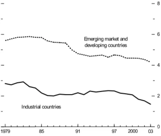
Stylized Facts Across Emerging Market and Developing Country Regions The volatility of per capita output growth in emerging market and developing countries has declined over the past three decades (Figure 1).3 However, it remains considerably higher than in industrial countries. Moreover, the decline in average volatility for all emerging market and developing countries taken together masks dif-ferent trends among regions.4 In particular, in south Asia and China, the Middle East and North Africa (MENA), and the CFA franc zone countries in sub-Saharan Africa, volatility has shown a sustained decline (Figure 2). In Latin America it has remained constant at a relatively high level, and in East Asia it has increased since 1997. Coun-tries in Asia have, on average, had the lowest, and counCoun-tries in sub-Saharan Africa the highest, volatility of the various emerging market and developing country regions over the 1970–2003 period. The transition economies in Central and Eastern Europe are excluded from the sample because a consistent set of macroeconomic data only became available after the transition to a market economy in the early 1990s. Figure 1 Volatility of Output Growth
(Rolling 10-year standard deviations of per capita real output growth rates; mean for each group)a
1979 85 91 97 03 0
2 4 6 8
Emerging market and developing countries
Industrial countries
2000
Note:a Data for 1979 refers to the standard deviation of per capita growrth rates for the period 1970–79. Data for 1980 does the same for the period 1971–80, etc.
Sources: Penn World Tables Version 6.1; and author´s calculations.
3 Output growth is defined as per capita real GDP growth. It is measured using data on real per capita GDP
in constant dollars (international prices, base year 1996) obtained from the Penn World Tables (PWT), Version 6.1. The PWT data covers the 1970–2000 period. Real per capita GDP growth rates calculated using data from the WEO database were used to extend the series to 2004.
4 The paper groups emerging market and developing countries into regions primarily according to their
geographic location: east Asia, south Asia and China, the Middle East and North Africa, Latin America, and sub-Saharan Africa. The latter region is further divided into CFA franc zone countries and non-CFA countries (see Appendix I for the countries included in each region). China is grouped with south Asia (because its cycle is more closely correlated with this region than with east Asia), but the results reported are not sensitive to China’s classification.
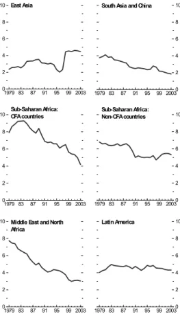
Table 1 reports averages of the output volatilities and worst output drops in each region for the 1970–86 and 1987–2003 periods, respectively. These subperiods are chosen because they capture a break in output volatility.5 The pattern of the aver-age volatilities across regions and from the first subperiod to the second is broadly consistent with the pattern observed based on the standard deviation of growth rates computed over a 10-year rolling window, suggesting that the analysis is not material-ly affected by the creation of two subperiods. The data on the worst output drops across regions reveals a pattern that is similar to the one for volatility: sub-Saharan Africa, south Asia and China, and the MENA region witnessed a decline in the se-verity of worst output drops from the first sub-period to the second, while the severi-ty of worst drops increased in east Asia and remained more or less the same in Latin America. In addition,the severity of worst output dropsis greatest in sub-Saharan Figure 2 Volatility of Output Growth by Regiona
(Rolling 10-year standard deviations of per capita real output growth rates; mean for each group)
1979 83 87 91 95 99 20030 2 4 6 8 10 1979 83 87 91 95 99 2003 0 2 4 6 8
10 East Asia South Asia and China
1979 83 87 91 95 99 20030 2 4 6 8 10 1979 83 87 91 95 99 2003 0 2 4 6 8
10 Sub-Saharan Africa: CFA countries Sub-Saharan Africa: Non-CFA countries
1979 83 87 91 95 99 2003 0 2 4 6 8 10 1979 83 87 91 95 99 20030 2 4 6 8 10 Latin America Middle East and North
Africa
Note:a See Appendix 1 for definition of country groups.
Source: Penn World Tables Version 6.1; and author´s calculations.
5 The analysis in the paper is broadly robust to changing the break date by one to two years in either
Table 1 Output Volatility and Output Drops by Region Volatility of Output
Growth Worst Drop of Output Growth
Volatility of Country--Component of Output Growth Worst Drop of Country-Component of Output Growth 1970−86 1987–2003 − 1970−86 1987–2003 − 1970−86 1987–2003 − 1970−86 1987–2003 − Sub-Saharan Africa CFA countries Mean 8.4 5.6 13.8 10.8 7.3 5.3 12.2 10.4 Min 4.1 2.4 29.1 28.2 2.3 1.8 28.5 28.1 Max 17.4 15.4 3.8 3.5 17.0 15.5 1.9 2.1 Std. Dev. 3.8 4.0 8.3 7.6 4.2 4.2 7.9 8.1 Non-CFA countries Mean 7.0 5.4 12.5 11.6 6.2 5.2 11.6 10.8 Min 2.0 1.5 29.1 34.9 1.6 1.2 29.0 34.6 Max 12.3 11.2 2.9 -0.6 10.2 11.0 1.7 0.6 Std. Dev. 2.9 3.2 6.9 9.5 2.6 3.2 6.8 9.0 Middle East and North Africa Mean 6.8 3.8 10.6 6.8 5.7 3.5 8.6 6.1 Min 3.2 1.2 24.8 15.8 2.9 1.1 20.0 11.9 Max 13.9 5.8 2.5 -0.8 10.8 5.7 1.4 0.3 Std. Dev. 3.9 1.6 7.9 5.0 2.9 1.5 5.9 4.0
Latin America Mean 4.7 4.7 8.6 8.3 4.0 4.3 6.8 7.4 Min 2.1 0.9 23.9 18.7 1.3 0.9 22.1 17.7 Max 7.3 13.6 1.2 0.8 7.1 12.7 -0.9 0.1 Std.
Dev. 1.4 3.1 5.4 5.3 1.5 2.8 5.2 4.8
East Asia Mean 3.2 4.0 3.1 7.0 2.3 2.2 1.5 0.1
Min 2.1 2.7 8.5 11.6 1.3 1.5 7.3 2.7
Max 4.0 5.0 -1.0 1.8 3.4 3.0 -1.9 -2.1 Std.
Dev. 0.8 1.0 3.3 4.0 0.8 0.6 3.6 1.8
South Asia
and China Mean 3.7 2.4 4.6 2.6 2.9 2.0 2.5 1.4
Min 2.5 1.4 11.5 5.9 1.8 1.3 7.7 4.3 Max 5.9 3.8 1.6 -0.2 5.2 3.1 0.0 -0.9 Std. Dev. 1.3 1.0 4.2 2.7 1.4 0.8 3.1 2.2 Emerging market and Developing Countries Mean 5.9 4.6 9.8 8.7 5.0 4.2 8.2 7.4 Min 2.0 0.9 29.1 34.9 1.3 0.9 29.0 34.6 Max 17.4 15.4 -1.0 -0.8 17.0 15.5 -1.9 -2.1 Std. Dev. 3.0 2.9 7.0 6.9 2.9 2.9 6.7 7.0 Industrial countries Mean 2.6 2.1 3.2 2.5 1.8 1.5 1.6 1.2 Min 1.8 1.5 8.1 7.6 0.9 0.7 7.1 4.7 Max 4.5 3.8 0.1 0.6 3.5 2.6 -1.0 -0.7 Std. Dev. 0.7 0.6 2.3 1.7 0.6 0.6 2.1 1.5
Notes: Output growth volatility is the standard deviation of real GDP per capita growth rate in each subperiod. The worst output drop is defined as the lowest annual GDP per capita growth rate in each subperiod. Volatility of country-component of output growth is the standard deviation of the country-specific com-ponent of per capita GDP growth as derived from the estimates of the dynamic factor model. The worst drop of the country-component of output growth is defined as the worst country-component of annual GDP per capita growth derived from the dynamic factor model in each subperiod. The sign of the worst drops is changed so that an output fall is a positive number.
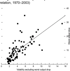
Africa and lowest for the countries in Asia. A plot of each country’s average vol-atility (excluding the worst drop) over the 1970–2003 period against the magnitude of the worst output drop confirms their strong correlation (Figure 3).6
What explains these regional differences in output volatility and the severity of worst output drops? To address this question, a dynamic factor model is estimated to decompose fluctuations in real per capita output growth. This technique allows one to identify and estimate common movements or underlying forces (“factors”) which may be driving output fluctuations across countries (see Appendix II for details). The dynamic factor model used in this paper decomposes output fluctuations into three factors:
– a global factor, which captures shocks that affect real per capita output growth in all countries;
– a regional factor,which captures shocks to real per capita output growth that are common to countries in a particular region;and
– a country-specific factor, which captures shocks to real per capita output growth that affect an individual country.7
Figure 3 Output Volatility and Worst Output Dropsa (Simple correlation, 1970–2003) 0 2 4 6 8 10 12 14 160 10 20 30 40 W or st out pu t dr op
Volatility excluding worst output drop
Note:a Output volatility is the standard deviation of annual real per capita GDP growth between 1970 and 2003. The worst output drop is each country´s worst annual real GDP per capita growth rate between 1970 and 2003. Sign of worst output drop has been changed so that a negative growth rate is a positive "output drop“.
Source: Author´s calculations.
6 The picture would not be too different if it plotted the output drops that exceed a 1.75 standard deviation
threshold against volatility excluding drops that exceed the 1.75 standard deviation threshold.
7 The country-specific factor is obtained as a residual after the global and regional factors are estimated.
The residual can therefore capture country factors as well as other factors. However, 15 alternative country groupings were explored, including groupings based on the level of development and structure of pro-duction (e.g., emerging market economies and oil and primary commodity exporting countries) and these did not reveal regional cycles as pronounced as those captured here, precluding the possibility that any quantitatively important factors were missed.
These “factors” capture movements in the underlying forces driving output fluctuations in these economies (i.e., monetary and fiscal policy shocks, oil price shocks, productivity shocks), the relative importance of which changes over time and can vary across countries. For example, the co-movement across countries of vari-ables affecting output growth, such as key international interest rates and oil prices, would be captured by the global factor. A shock that spills over from one country in a region to another owing to similarities in the quality of economic and political in-stitutions or the stage of economic development, would be captured by the regional factor. Changes in macroeconomic policy implementation or structural reforms which affect the volatility of output growth in a particular country would be captured by the country-specific factor.8
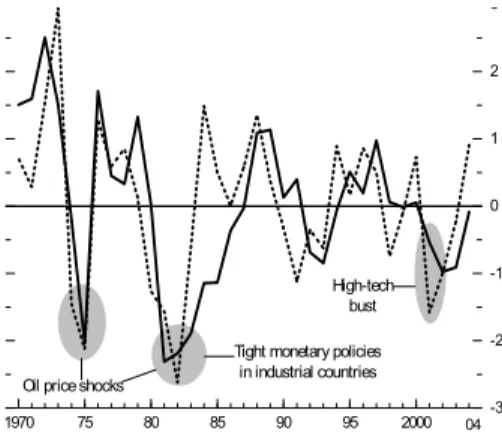
The estimate of the global factor picks up the key peaks and troughs in global GDP growth from 1970 to 2004, including the oil price shocks in the 1970s, the re-cessions in the early 1980s and 1990s, and the high-tech investment bust in the early 2000s (Figure 4). As is the case with actual global growth, the global factor ( ftGlobal) is less volatile during the second half of the sample period.
The estimates of the regional factors also capture well-known cyclical fluc-tuations (Figure 5).9 For example, the east Asia factor shows that the crisis in 1997–98 Figure 4 Global Factor and Actual Global Growth
(Annual percentage change; deviation from sample meen)
1970 75 80 85 90 95 2000 -3 -2 -1 0 1 2 3 04
Oil price shocks
Tight monetary policies in industrial countries
High-tech bust
Notes:
global factor – See Appendix 2 for further details on the estimation of the global factor. The global fac-tor has been rescaled to have the same variance as the actual global (fGlobal) growth.
actual global growth – represents the purchasing-power-parity-weighted real per acpita GDP growth rates for all countries in the study.
Source: Penn World Tables Version 6.1; and author´s calculations
8 If a country is heavily dependent on a particular commodity, either as an exporter or as an importer,
an externally driven change in the price of that commodity could be captured by the country-specific factor as well.
9 In addition to the regional groupings described in footnote 4 for the estimation of the dynamic factor
model, Latin America is further subdivided into Central America and the Caribbean, and South America, and the industrial countries are subdivided into G-7 and other industrial countries to capture differences in their regional cycles.
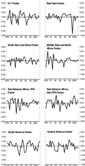
dominates the cycle in the region; the South America factor captures the debt crisis in the early 1980s, the high inflation of the late 1980s, and the problems of the late 1990s; and the CFA factor exhibits sharp swings in the 1970s and early 1980s, re-flecting the recurrence of droughts and terms of trade shocks, but has been less vola-tile recently. Some of the regional factors, however, exhibit no distinguishable cycles.
To investigate the importance of each of the three factors for explaining out-put volatility in each country, we calculate the share of the variance of real per ca-pita output growth that is due to each. The results suggest that output fluctuations in Figure 5 Regional Factorsa
(Annual percentage change, deviation from sample meen)
1970 75 80 85 90 95 2000 -0.08 -0.06 -0.04 -0.02 0.00 0.02 0.04 0.06 G-7 Factor 1970 75 80 85 90 95 2000 -0.08 -0.06 -0.04 -0.02 0.00 0.02 0.04 0.06
East Asia Factor
1970 75 80 85 90 95 2000 -0.08 -0.06 -0.04 -0.02 0.00 0.02 0.04 0.06 1970 75 80 85 90 95 2000 -0.08 -0.06 -0.04 -0.02 0.00 0.02 0.04 0.06 1970 75 80 85 90 95 2000 -0.08 -0.06 -0.04 -0.02 0.00 0.02 0.04
0.06 South Asia and China Factor
1970 75 80 85 90 95 2000 -0.08 -0.06 -0.04 -0.02 0.00 0.02 0.04 0.06 1970 75 80 85 90 95 2000 -0.08 -0.06 -0.04 -0.02 0.00 0.02 0.04 0.06 Sub-Saharan Africa: Non-CFA Factor Sub-Saharan Africa: CFA
Factor 1970 75 80 85 90 95 2000 -0.08 -0.06 -0.04 -0.02 0.00 0.02 0.04 0.06
Middle East and North Africa Factor
Central America Factor South America Factor
Note:a See Appendix 2 for further details on the estimation of the regional factors. A other industrial countries factor is also estimated bur is not schown here.
emerging market and developing countries have been driven more by country-spe-cific factors than those in industrial countries (Figure 6). For example, the country- -specific factor explains more than 60 percent of output volatility in about 90 percent of emerging market and developing countries, compared with only 40 percent of in-dustrial countries. The global factor explains less than 10 percent of output fluc-tuations for more than 60 percent of the emerging market and developing countries, but between 10 and 20 percent of the output variation in nearly half the industrial countries.
An examination of the contributions of the factors to output volatility shows that in all the emerging market and developing country regions, except east Asia, at least 60 percent of output volatility has been attributable to country-specific factors (Table 2). Also, unlike in industrial countries, in all emerging market and developing country regions the regional factor has explained a greater fraction of volatility than the global factor. The contribution of the country-specific factor for explaining output fluctuations in east Asia has been about the same as for industrial countries, while the contribution of the regional factor has been very large, mainly reflecting the ef-fects of the east Asian financial crisis, which resulted in large output losses across the region. Indeed, estimating the model over the 1970–96 period suggests a more prominent role for the global factor and a less prominent role for the regional factor, making East Asia resemble more closely the pattern observed in industrial countries. Figure 6 Contributors to Volatility in Real per Capita Outup Growth, 1970–2004a
(Percent of countries on y-axis, x-axis as stated) Global Regional Country
10 20 30 40 50 60 70 80 90 100 0 10 20 30 40 50
Percent explained by factor Industrial Countries 10 20 30 40 50 60 70 80 90 100 0 10 20 30 40 50 60 70
Percent explained by factor Emerging Market and Developing Countries
Note:a Twenty percent explained by a factor refers to countries for which between 10 and 20 percent of varia-tions on output are explained by the factor; 30 percent refers to countries for which between 20 and 30 percent of variations are explained by the factor, and so on.
To investigate the reasons for the trend decline in output volatility in most of the emerging market and developing country regions the dynamic factor model is estimated over two periods: 1970–86 and 1987–2004 (Table 3).10 The results suggest that the declines in output volatility in emerging market and developing country re-gions have been mainly due to less volatile country-specific factors.11 In all regions, except Latin America, at least 70 percent of the decline in the variance of output growth has been explained by the country-specific factor. By contrast, for industrial countries, the corresponding share has been about 50 percent.12
Table 2 Contributors to Volatility in Real Per Capita Output Growtha (Averages for each group; in percent)
Global Regional Country Sub-Saharan Africa
CFA countries 5.7 18.2 76.1
Non CFA countries 6.8 10.2 82.1
Middle East and North Africa 3.8 15.9 80.3
Latin America 12.6 13.7 73.7
South Asia and China 15.6 20.6 63.8
East Asia 11.0 41.8 47.2
East Asia (1970−96) 18.0 15.8 66.3
Developing countries 9.3 16.9 73.8
Industrial countries 24.3 21.7 54.0
Note:a The table shows the fraction of the variance in real per capita output growth attributable to each factor. Table 3 What Explains the Declines in Output Volatility Between 1970−86 and
1987−2004? a
(Averages for each group; in percent)
Decline in Variance
of Output Growth Global Regional Country Sub-Saharan Africa
CFA countries -40.0 -2.1 -5.8 -32.1
Non-CFA countries -53.2 -6.9 -8.3 -38.0
Middle East and North Africa -60.7 -0.5 -17.4 -42.7
Latin America -12.1 -3.4 -2.8 -5.9
South Asia and China -12.0 -0.9 -2.9 -8.2
Developing countries -34.2 -3.2 -6.8 -24.2
Industrial Countries -4.1 -1.1 -0.8 -2.3
Note:a Only countries which experienced a decline in volatility from the 1970−86 period to the 1987−2004 period are included in the calculations. For this reason countries in East Asia are not included. The ta-ble shows the contribution of each factor to the decline in the variance of output growth from the 1970− –86 period to the 1987−2004 period.
10 Recent work by Kose, Otrok, and Whiteman (2003) uses this technique to examine changes in
the business cycles of G-7 countries.
11
Table 3 reports results in countries where volatility has declined. It therefore differs from Figure 2,
which shows average volatility for all countries in a region. This difference is particularly important for sub-Saharan Africa’s non-CFA countries, a number of which experienced large increases in volatility during the 1987–2004 period.
12 The volatility of the country component of output growth in each subperiod and the worst drop of
the country component of output growth in each subperiod are shown in Table 1. The volatility of the
coun-try component of output growth declined for all regions except Latin America. Another interesting ob-servation is that for east Asia, while overall volatility increased in the 1987–2003 period, the volatility of the country component of output growth declined.
An analysis of the worst output drops in emerging market and developing country regions suggests that they have been mainly associated with country-specific events. The exception to this pattern is East Asia, where the regional factor has been the main contributor to the worst drops (Table 4). The results also show that the con-tribution of the country-specific factor to the worst output drops in emerging market and developing country regions increased from the first to the second subperiod. In line with these observations and the decline in worst overall output drops, Table 1 shows that the worst drop of the country component of output growth declined on average from the first subperiod to the second in all emerging markets and develop-ing country regions except Latin America. By contrast, the global factor was the main factor contributing to the worst output drops in industrial countries in the 1970–86 period, accounting on average for 70 percent of the worst drops, and the regional factor was the main contributor to the worst drops in the 1987–2003 period.13 3. Cross-Section Determinants of Output Volatility and Output Drops 3.1 Methodology and Data
This section reports the estimation results for cross-section regressions of out-put volatility and worst outout-put drops. Dependent variables are defined in two ways. In one set of regressions, they are defined as the standard deviation of real per capita GDP growth and the worst drops in real per capita output growth over the 1970–2003 period. In a second set, dependent variables are defined as the standard deviation of the country-specific component of real per capita GDP growth for the 1970–2003 pe-riod and the worst drop in the country-specific component of output growth over the 1970–2003 period from the dynamic factor analysis.
The explanatory variables in the regressions are similar to those that have been used in other studies examining output volatility (e.g., Easterly, Islam, and Stig-litz, 2000; and Kose, Prasad, and Terrones, 2003). These variables consist of: an in-Table 4 Worst Output Drops: Global, Regional, and Country Factors a
(Averages for each group; in percent)
1970–1986 1987–2003
Global Regional Country Global Regional Country Sub-Saharan Africa
CFA countries 4.9 27.7 67.5 2.6 8.9 88.5
Non-CFA countries -1.8 11.1 90.7 -14.7 -1.8 116.4 Middle East and North Africa 6.0 16.9 77.1 9.9 15.1 74.9
Latin America 24.1 11.5 64.5 1.2 10.2 88.6
South Asia and China 35.0 30.5 34.6 -113.5 10.6 202.9
East Asia 50.0 120.5 -70.5 7.9 104.5 -12.4
Emerging market and 15.0 27.5 57.6 -9.6 18.5 91.1 developing countries
Industrial countries 71.6 46.1 -17.8 20.7 59.5 19.8
Note:a The table shows the contribution of each factor to the worst drop in real per capita output growth. The worst output drop is defined as the lowest annual GDP per capita growth rate in each subperiod.
13 The growing importance of the regional factor in driving output drops and volatility is consistent with
the finding of an increased degree of synchronization of business cycles across industrialized countries over time (see for example Bordo and Helbling, 2003; and Kose, Otrok, and Whiteman, 2003).
dicator of the volatility of discretionary government spending, an indicator of the pro-cyclicality of fiscal policy, terms of trade volatility, the interaction of exchange rate flexibility with terms of trade volatility, relative income, trade openness, an indicator of financial sector development, and an indicator of capital account restrictions. Data sources and variable definitions are discussed in Appendix 3.
The estimation focuses, in particular, on identifying the effects of fiscal policy and terms of trade volatility in conjunction with exchange rate policy on output vola-tility and worst output drops. The paper builds on the finding by Fatás and Mihov (2003) of a robust negative relationship between output volatility and discretionary fiscal policy volatility.14 The paper replicates this finding for output volatility and ex-tends the analysis to the new measure of country-specific output volatility as well as the two measures of worst output drops. The paper also examines the relationship be-tween fiscal policy procyclicality and output volatility and worst output drops.
In order to investigate whether the exchange rate regime affects output vola-tility and the magnitude of the worst drops, the regressions include an indicator of ex-change rate flexibility and the interaction of terms of trade volatility with the variable capturing the flexibility of the exchange rate regime. The indicator of exchange rate flexibility is based on the de facto “natural classification” developed by Reinhart and Rogoff (2004).
The specification of the regressions for output volatility and worst output drops are broadly the same. The explanatory variables are averages over the 1970–2003 pe-riod. For the worst output drop regressions, exchange rate flexibility is captured by the index of flexibility in the year prior to the drop, while relative income is meas-ured at the beginning of the sample period (rather than averaged over the period). An important specification issue that arises relates to the possibility of reverse cau-sation and simultaneity of the fiscal policy variables. Following Fatás and Mihov, the regressions use political and institutional variables to instrument for the potential endogeneity of the fiscal policy variables (building on the notion that politically constrained policymakers generate lower volatility). The political and institutional indicators used as instruments include the nature of the electoral system (majoritarian versus proportional) and the nature of the political system (presidential versus parlia-mentary). It is expected that majoritarian voting rules and a parliamentary form of government would be associated with lower fiscal volatility.15
The variables used in the cross-section regression analysis, grouped by region, are presented in Appendix 3. Sub-Saharan African countries had the highest volatility of output growth, the most severe worst drops in output, the highest volatility of dis-cretionary government spending, and the highest terms of trade volatility, on average, 14 The measure of fiscal policy volatility used in the regressions is the same as the one used by Fatás
and Mihov, namely, the standard deviation of the residual from an instrumental variables regression of the growth of government spending on output growth, a one-period lag of the growth of government spending, a time trend, and various control variables.
15 There are also endogeneity issues associated with the trade openness and financial sector development
variables in the regressions. The instrumental variables regressions therefore instrument for these variables using the predicted trade to GDP ratios as constructed by Frankel and Romer (1999), variables which capture whether the legal system in a particular country has its origin in either the French, English, or German system, life expectancy, and the number of political assassinations per million (e.g., Easterly, Islam, and Stiglitz, 2000).
over the 1970–2003 period. For example, Guinea-Bissau, which had the largest out-put contraction in the sample (29 percent in 1970) and the highest volatility of outout-put growth (16 percent), had high discretionary government spending volatility and terms of trade volatility even compared with other sub-Saharan African countries. In con-trast, East Asia had the lowest volatility of the country component of output growth and the smallest worst drop of the country component of output among emerging market and developing countries, and also had the lowest volatility of discretionary government spending and was subject to smaller terms of trade shocks. There was not much variation in average exchange regime flexibility over the sample period across several of the emerging market and developing country groups; average ex-change regime flexibility varied across the countries in each regional group. CFA franc zone countries had the lowest exchange regime flexibility on average, while sub-Saharan Africa’s non-CFA countries had the highest exchange regime flexibility. 3.1 Results
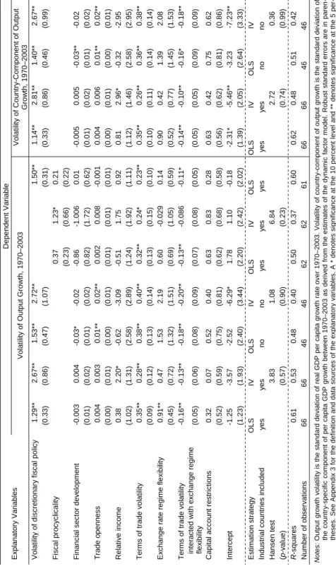
Table 5 reports the results from ordinary least squares and instrumental vari-ables estimation of the cross-section regressions of output volatility. Due to data availability, the regressions use data from 46 developing countries and 20 industrial countries. Robust standard errors are reported in parentheses. Hansen J tests of overidentifying restrictions in the instrumental variable estimations do not reject the econometric specification and the validity of the instruments. The findings from the regressions that use the standard deviation of the country-specific component of output volatility derived from the dynamic factor model as the dependent variables (last four columns) are broadly the same in magnitude and significance as those which use overall output volatility as the dependent variable. Three variables – volatility of discretionary government spending, terms of trade volatility, and the interaction of terms of trade volatility with the index of exchange regime flexibility – are found to be the key determinants of output volatility and worst output drops; the other explan-atory variables are, for the most part, insignificant.
The volatility of discretionary fiscal policy is found to have a strong positive and significant effect on the two measures of output volatility. This finding is robust to excluding the industrial countries from the sample. The magnitude of the effect of discretionary fiscal spending volatility on output volatility is larger in the instrumen-tal variable (IV) regressions, suggesting a strong effect of discretionary fiscal policy on the volatility of both output growth and the country-specific component of output growth.
Terms of trade volatility is also found to have a positive and significant effect on output volatility. The exchange rate regime itself is not a significant determinant in nearly all the regressions. However, the interaction of terms of trade volatility with the variable capturing the flexibility of the exchange rate regime during the sample period is negative and significant, confirming that the association between terms of trade shocks and output volatility is more pronounced under fixed than flexible ex-change rate regimes. These results are also robust to the exclusion of the industrial countries from the sample. For example, the estimates from the regression of the vola-tility of the country component of output growth for the sample of emerging market and developing countries suggest that a one standard deviation increase in terms of trade volatility implies a 1.5 percentage point increase in output volatility in the re-
Table 5 V
o
latility of Output Gro
w th : R e gression R e sults Dependent Varia b le Ex planatory Variables Volatili ty of Output Grow th, 19 70–200 3 Volatili ty of Cou n tr y -Component of Ou tput Grow th, 19 70–200 3 Volatili ty of discre ti onary fiscal poli c y 1.29 ** 2. 67 ** 1.53 ** 2.72 ** 1.50 ** 1.14 ** 2.81 ** 1.40 ** 2.67 ** (0.33) (0.86) (0.47) (1.07) (0 .31) (0.33) (0.86) (0.46) (0.99) Fiscal pro c y c licali ty 0.37 1.23 * 0.21 (0.23) (0.66) (0.22) Financial se ctor de v e lopment -0.003 0.004 -0.03 * -0.02 -0.86 -1.006 0.01 -0 .005 0.005 -0.03 ** -0.02 (0.01) (0.02) (0.01) (0.02) (0.82) (1. 72) (0.62) (0.01) (0.02) (0.01) (0.02) Trade openn ess 0.004 0.003 0.01 ** 0.02 ** 0. 002 0.008 -0.001 0.004 0.006 0.01 ** 0.02 ** (0.00) (0.01) (0.00) (0.01) (0.01) (0. 01) (0.01) (0.00) (0.01) (0.00) (0.01) Relativ e income 0.38 2.20 * -0.62 -3. 09 -0.51 1.75 0.92 0.81 2.96 * -0.32 -2.95 (1.02) (1.31) (2.58) (2.89) (1.24) (1. 92) (1.11) (1.12) (1.46) (2.58) (2.95) Terms o f trade v o latility 0.35 ** 0.28 ** 0.38 ** 0. 40 ** 0.32 ** 0.24 * 0.23 ** 0.35 ** 0.26 ** 0.36 ** 0.38 ** (0.09) (0.12) (0.13) (0.14) (0.13) (0. 15) (0.10) (0.10) (0.11) (0.14) (0.14) Ex change ra te r egi me flex ibility 0.91 ** 0.47 1.53 2.19 0.60 -0.029 0. 14 0.90 0.42 1.39 2.08 (0.45) (0.72) (1.32) (1.51) (0.69) (1. 05) (0.59) (0.52) (0.77) (1.45) (1.53) Terms o f trade v o latility -0.16 ** -0.1 3 ** -0.18 ** -0.20 ** -0.13 ** -0.086 -0.1 1 * -0.14 ** -0.10 ** -0.16 * -0.18 ** intera cted w ith ex change re gime flex ibility (0.05) (0.06) (0.08) (0.09) (0.07) (0. 08) (0.05) (0.05) (0.05) (0.09) (0.09) Capital accoun t restrictio n s 0.32 0.07 0.52 0.40 0.63 0.83 0.28 0.63 0.42 0.75 0.62 (0.52) (0.59) (0.75) (0.81) (0.62) (0. 68) (0.58) (0.56) (0.62) (0.81) (0.86) Inte rcep t -1.25 -3.57 -2.52 -6.29 * 1.78 1.10 -0.18 -2.31 * -5.46 ** -3.23 -7.23 ** (1.23) (1.93) (2.40) (3.44) (2.20) (2. 42) (2.02) (1.39) (2.05) (2.64) (3.33) Estimation stra tegy OLS IV OLS IV OLS IV OLS OLS IV OLS IV Indu stri al coun trie s included y e s y e s no no y e s y e s y e s y e s y e s no no Hansen te st 3.83 1. 08 6.84 2.72 0.36 ( p -v alue) (0.57) (0.90) (0.23) (0.74) (0.99) R -square s 0.61 0.53 0.48 0.40 0. 50 0.37 0.60 0.62 0.48 0.51 0.42 Number of ob serv ation s 66 66 46 46 62 62 61 66 66 46 46 Notes: Out put gro w th v o la tilit y is the sta n dard de v iat ion of real
GDP per capita gro
w th rate o v er 19 70– 2003. Vol a tilit y of co untr y -co mpon
ent of output gro
w th is the standar d de v iati on of the countr y -s pecifi c compon ent of per ca pita GDP gro w th bet w e en 1970 –200 3 as deri v ed from th e esti mates of the d y na mi c factor m odel. Rob u s t standard erro rs ar e in paren-theses. See Appe ndi x 3 for t he d e finiti on and da ta so urces of the e x pl anat or y v a ri a b les. A * den otes sig n ificanc e at t he 10 p e rcent l e v e l a nd ** d enotes signifi cance a t the 5 per-cent le vel. IV i n strum ents the v o lati lit y of f iscal poli c y , fin ancial sector d e v elo p ment and tra de to GDP va riables (s ee te xt f or f u rther e x plan ation).
gion with the least exchange rate flexibility (the CFA franc zone) compared with a 0.3 percentage point increase in the region with the greatest exchange rate flexi-bility (non-CFA countries).
With a few exceptions, the other explanatory variables in the regressions for the total sample are insignificant. Unlike previous work, the financial sector devel-opment variable is positive but not significant in the IV regressions for the entire sample of countries. The sign of the coefficient is negative in the regressions which exclude industrial countries but it is only significant in the OLS regressions.16 The trade and capital account restrictions variables are positive but not statistically significant in the regressions for the entire sample of countries. The coefficient on trade openness is found to be positively and significantly associated with country- -specific and overall output volatility but only in the regressions that exclude indus-trial countries.17, 18
Table 6 reports the results of the regressions for the worst output drops. Due to data availability, the regressions use data from 43 (44, in some cases) emerging market and developing countries and 20 industrial countries. A parsimonious spe-cification is estimated for the instrumental variables regressions of the worst drop of the country component of output growth. The results broadly mirror those for the vol-atility regressions. The volvol-atility of discretionary spending variable is found to be a significant determinant of worst output drops in the ordinary least squares and instrumental variables regressions for the entire sample of countries. The magnitudes of the coefficients on volatility of discretionary government spending are much larger in the instrumental variables regressions of the overall and country-specific compo-nent of worst output drops. The fiscal policy procyclicality variable is not found to have a significant effect on worst output drops, irrespective of whether discretionary fiscal volatility is included as another explanatory variable and/or whether the vari-able is instrumented. This lends support to the notion that what matters most for the severity of the worst output drops is the volatility of discretionary government spending. This finding is robust to excluding industrial countries.
Terms of trade volatility is also found to be a significant determinant of worst output drops. As was the case in the regression for output volatility, its impact is dampened in countries with flexible exchange rate regimes. The indicator of exchange rate regime flexibility is found to have a positive and significant effect on worst output drops in the regression of the worst drop of overall output growth. However, this finding is not robust to the exclusion of outliers from the worst output drop regressions.19 Moreover, the indicator of exchange rate flexibility is not found to 16 The financial sector development variable is, however, found to be negative and significant in
re-gressions that do not control for discretionary fiscal policy volatility (not shown in tables).
17 This finding may be consistent with trade having a differential effect on countries depending on whether
they engage in intra- or inter-industry trade. Recent work has shown, however, that countries that are more open to trade can tolerate higher volatility without hurting their long-term growth (Kose, Prasad, and Terrones, 2003).
18 The volatility regression results are also robust to the inclusion of indicators of institutional quality from
the International Country Risk Guide constructed as the average of indicators of corruption, rule of law, and the quality of the bureaucracy over the 1984–2003 period (not shown here).
19 Outlying observations are defined here as the two countries included in the regression sample with
Table 6 Worst Output Dr ops : Regre ssion Re sults D epe nd ent V a ri ab le Ex plana tory V a ria b le s O u tpu t G row th B e tw een 1 9 7 0 a n d 2 003 Wo rs t D rop of C o unt ry -C o mpon ent of O u tp ut G row th B e tw een 197 0 an d 2 0 0 3 V o lati lity of d is c re ti on ary fisc al po licy 2.0 3 ** 4.2 1 * 2.3 1 8.8 3 ** 2.2 8 ** 2.1 9 ** 2.6 1 ** 4.5 6 ** 2.5 7 * 5.9 7 * (0. 99) (2. 47) (1. 59) (4. 12) (0. 98) (0. 99) (0. 92) (1. 73) (1. 46) (3. 1 7) F isca l p ro c y c lical it y -0. 23 0.5 8 -0. 68 (0. 73) (1. 64) (0. 73) F inan ci al se cto r d e v e lopme n t -0. 0 0 8 0.0 10 -0. 03 0.0 3 -1. 09 0.4 1 -0. 36 -0. 02 (0. 02) (0. 04) (0. 05) (0. 05) (2. 11) (3. 75) (2. 04) (0. 02) T rade o p e n n e s s 0.0 01 -0. 0 0 6 0.0 0 0.0 0 -0. 0 0 3 0.0 05 0.0 1 0.0 1 (0. 01) (0. 02) (0. 01) (0. 02) (0. 02) (0. 03) (0. 02) (0. 01) R e lativ e in com e i n 19 70 -1. 15 0.8 2 -2. 97 -8. 85 -7. 20* * -6. 12 -5. 05* * 2.6 6 1.4 9 4.8 6 2.0 4 -0. 0 3 (2. 33) (3. 26) (5. 33) (7. 34) (2. 40) (4. 38) (2. 46) (2. 86) (2. 25) (3. 11) (5. 69) (6. 7 6) Te rm s o f tr ad e v o la ti lit y 0 .95 ** 0 .83 ** 1 .16 ** 1 .28 ** 0 .91 ** 0 .85 ** 0 .86 ** 0 .78 ** 0 .85 ** 0 .74 ** 0 .93 ** 0 .90 ** (0. 23) (0. 24) (0. 28) (0. 31) (0. 26) (0. 28) (0. 25) (0. 23) (0. 20) (0. 21) (0. 27) (0. 2 6) Ex chan ge rat e re g ime fl ex ibility in y ear pri o r to w o rst dr op 2 .43 * 2 .04 * 4 .21 * 6 .31 ** 2 .66 ** 2 .01 2 .82 ** 0 .87 1 .33 1 .22 1 .95 2 .86 (1. 05) (1. 19) (2. 29) (3. 19) (1. 35) (1. 70) (1. 23) (1. 13) (1. 03) (1. 04) (2. 07) (2. 4 9) Terms of t ra d e v o latili ty inter a c te d wi th -0. 29* * -0. 25* * -0. 40* * -0. 49* * -0. 32* * -0. 28* * -0. 31 -0. 18* -0. 21* * -0. 19* * -0. 25* * -0. 28* * ex chang e re gime flex ibility pri o r to dro p (0. 10) (0. 10) (0. 14) (0. 18) (0. 11) (0. 13) (0. 11) (0. 09) (0. 08) (0. 07) (0. 12) (0. 1 3) C apit a l ac co unt r e stri cti o n s -0. 98 -1. 63 -1. 35 -3. 77 -0. 93 -0. 53 -1. 33 0.9 1 (1. 85) (1. 81) (2. 40) (2. 79) (1. 88) (1. 89) (1. 76) (2. 32) Int e rc ep t -2. 93 -6. 30 -6. 08 -22 .5 8 ** 4.0 6 2.8 5 -1. 21 -4. 94 -6. 05* -10 .0 3 -7. 37 -15 .6 0 (4. 12) (6. 50) (7. 05) (11 .7 1 ) (4. 45) (4. 77) (4. 74) (4. 42) (3. 36) (4. 49) (6. 07) (9. 9 0) Es ti ma ti o n st ra tegy OL S I V OL S I V OL S I V OL S OL S OL S I V OL S I V Ind u st ri al co unt rie s in cl ud ed y e s y e s no no y e s y e s y e s y e s y e s y e s no no H ans en te st 8.8 3 7.2 0 9.0 2 8.9 1 6.5 0 ( p -v alue ) (0. 12) (0. 13) (0. 11) (0. 11) (0. 1 6) R-s q u a re s 0 .57 0 .54 0 .42 0 .21 0 .49 0 .48 0 .55 0 .62 0 .63 0 .60 0 .48 0 .42 N u mber of o b s e rv atio ns 63 63 43 43 60 60 59 63 64 64 44 44 No te s: T h e w o rst out put d rop is d e fi ned a s t he w o rs t ann ua l G D P per c apit a grow th rat e betw een 1 9 7 0 – 2 0 03. T he w o rs t d ro p of th e co unt ry -compo ne nt of out -put grow th i s de fi ned as the w o rs t cou n tr y -compo n e n t of an nu al G D P per ca pit a gr ow th be tw een 1 9 7 0 – 200 3. T h e si gn of the w o rst d ro p s has be en cha n g e d s o th at an out pu t fa ll i s a po sitiv e num be r. S ee A p p e n d ix 3 f o r t he de fin iti on a nd dat a s o u rc e s of t he ex plana to ry v a ri able s. R o b u st sta n d a rd err o rs a re in pa re n-t h e s e s . A * de n o te s s ig n ifi c a n c e at t he 10 p e rc en t l e v e l and ** d e no te s sig n if ic an ce at the 5 pe rc ent lev e l. IV i n s trum e n ts th e v o lati lity of f is c al po licy , fin anc ial s e ct or d e v e lopm ent a n d tra d e to G D P v a riabl es (se e t e x t for fur th e r ex plan ati o n ).
have a significant effect in the regressions of the worst drop of the country compo-nent of output growth. The instrumental variable regression of the worst drop of the country component of output growth supports the idea that the impact of terms of trade volatility on output is dampened by the degree of exchange rate flexibility for the sample of emerging market and developing countries. For example, the esti-mations suggest that a one standard deviation increase in terms of trade volatility implies a 5 percentage point increase in the worst output drop in the region with the least exchange rate flexibility (the CFA franc zone) compared with a 3 percentage point increase in the region with the greatest exchange rate flexibility (sub-Saharan Africa’s non-CFA countries). The remaining variables including the financial sector development, trade openness, and capital account restrictions variable are not sta-tistically significant in any regression.
In order to understand the implications for output growth volatility of the changes in the main policy-driven factor, the impact on output volatility of reducing discre-tionary government spending volatility in each region is calculated. The estimates from the IV regression of the volatility of the country component of output growth for the emerging market and developing countries suggest that less volatile fiscal spending could have played a significant role in reducing output volatility in sub- -Saharan Africa during the sample period. Specifically, a reduction in the volatility of cyclically adjusted government spending to the level in East Asia would have reduced output volatility by 3.8 percentage points for countries in the CFA franc zone and by 3.1 percentage points for the non-CFA countries (Figure 7). These are
Figure 7 Output Volatility and Reduction in Volatility of Discretionary Fiscal Policya
-5.0 -4.5 -4.0 -3.5 -3.0 -2.5 -2.0 -1.5 -1.0 -0.5 0.0 0.5 1.0 R ea l G D P pe r ca pi ta gr owt h r at e v o la ti lit y Sub-Saharan Africa: CFA countries Sub-Saharan Africa: Non-CFA countries Latin America Middle East and North Africa South Asia and China East Asia Sub-Saharan Africa: CFA countries Latin America
Sub-Saharan Africa: Non-CFA countries Middle East and North Africa South Asia and China
Notes:a Figure schows change in standard deviation of average annual real GDP per capita growth if a parti-cular region reduced the volatility of fiscal discretionary policy to match the quality of other regions. Volatility of discretionary fiscal policy is measured as the standard deviation of the cyclically adjusted government spending estimated for the 1960–2000 period (se Fatás and Mihov, 2003). See Ap-pendix 1 for definition of country groups.
equivalent to about 50 and 60 percent of the country-specific output volatility respec-tively. Countries in other regions (most notably in Latin America) also stand to gain from a more stable fiscal policy.
4. Summary and Conclusions
Output volatility, including from large output drops, tends to have negative effects on long-term economic growth, welfare, and income inequality, particularly in developing countries. Reducing such volatility can therefore make an important contribution to improving growth and welfare. Although output volatility and large output drops have been on a downward trend in most emerging market and develop-ing country regions over the past three decades, they have remained higher than in industrial countries. This paper has shown that much of the output volatility in emerging market and developing countries has been driven by country-specific factors, underscoring the key role of domestic policies. The worst output drops in emerging market and developing countries also have been primarily associated with country-specific events. Thus, while emerging market and developing countries have made important strides in strengthening macroeconomic and structural policies in recent years, the remaining gap between their output volatility and that of developed countries suggests that more gains can still be made.
Several studies on international business cycles have focused on the impact of the increased globalization in recent decades on the synchronization of output fluctuations across countries. The results of the dynamic factor analysis used in this paper provide an interesting new perspective to this literature. The recent declines in output volatility and moderation of worst output drops in emerging market and developing countries have not been associated with greater relative contributions of global and regional factors to output volatility, as one would have expected with in-creased global linkages, but rather with more stable country specific factors. This finding suggests that the channel through which stronger trade and financial linkages may have contributed to lowering output volatility in emerging market and develop-ing countries is through encouragdevelop-ing a strengthendevelop-ing of domestic economic policies and institutions.
The evidence from the cross-section regressions suggests that volatility of dis-cretionary government spending, and terms of trade volatility, in conjunction with exchange rate flexibility, were key determinants of country-specific volatility and large output drops during the 1970–2003 period. Discretionary fiscal policies tended to increase volatility and the severity of output drops, particularly in sub-Saharan Africa and Latin America. To contain the volatility of fiscal policies, greater expend-iture restraint during cyclical upturns would have been beneficial. The strengthening of budgetary institutions would also be helpful; while several emerging market and developing countries have adopted fiscal responsibility laws to constrain discretion in government spending in recent years, the effectiveness of such laws remains an em-pirical issue. Terms of trade volatility is associated with more severe worst output drops and higher volatility of output growth. The paper also illustrates that exchange rate flexibility may cushion the impact of terms of trade shocks on output drops and output volatility. Interestingly, while previous work has found a role for financial sector development, the evidence presented here suggests that its effect on output volatility is not robust to the inclusion of variables related to fiscal policy volatility.
APPENDIX 1
Regional Groupings and Country Coverage
In addition to the regional groupings mentioned in section 2 (footnote 4), the estimation of the dynamic factor model was done by further subdividing Latin America into (1) Central America and the Caribbean and (2) South America, and the industrial countries into (1) G-7 and (2) other industrial countries.
The grouping of the countries by region appears to be well-suited to identify a “regional factor” because countries that are geographically close to each other are likely to be affected by the same shocks, such as weather-related shocks or terms of trade shocks. In addition to the geographic aspect of the groupings, other factors such as trade and financial linkages or a degree of policy coordination (e.g., the longstand-ing peg of the CFA franc zone countries, initially to the French franc and now to the euro) can justify common regional cycles. The justification for grouping the in-dustrial countries together is not based on geography but rather reflects the size of their economies, their stage of economic development, and the quality of their in-stitutions.
Industrial countries
G-7 countries. Canada, France, Germany, Italy, Japan, the United Kingdom, and the United States.
Other industrial countries. Australia, Austria, Belgium, Denmark, Finland, Greece, the Netherlands, New Zealand, Norway, Portugal, Spain, Sweden, and Switzerland.
Latin America
Central America and the Caribbean. Costa Rica, Dominican Republic, El Salvador, Guatemala, Guyana, Haiti, Honduras, Mexico, Nicaragua, Panama, and Trinidad and Tobago.
South America. Argentina, Bolivia, Brazil, Chile, Colombia, Ecuador, Para-guay, Peru, UruPara-guay, and Venezuela.
Middle East and North Africa (MENA)
Algeria, Egypt, Iran, Israel, Jordan, Morocco, Syria, Tunisia, and Turkey. Sub-Saharan Africa
CFA franc zone countries. Burkina Faso, Cameroon, Republic of Congo, Côte d’Ivoire, Gabon, Guinea-Bissau, Mali, Niger, Senegal, and Togo.
Non-CFA countries. Botswana, Burundi, Ethiopia, Gambia, Ghana, Kenya, Madagascar, Malawi, Mozambique, Namibia, Nigeria, Sierra Leone, South Africa, Tanzania, Uganda, and Zambia.
South Asia and China
Bangladesh, China, India, Pakistan, and Sri Lanka. East Asia
APPENDIX 2
The Dynamic Factor Model
Dynamic factor models are a generalization of the static factor models com-monly used in psychology. The motivation underlying these models, which are gain-ing increasgain-ing popularity among economists, is that there are a few common factors that are driving fluctuations in large cross sections of macroeconomic time series. While these factors are unobservable and cannot be identified as clearly “productivity shocks” or “monetary shocks,” the rationalization for these models is that a few ag-gregate shocks are the underlying driving forces for the economy. The unobserved factors are then indexes of common activity. These factors can capture common activity across the entire dataset (e.g., global activity) or across subsets of the data (e.g., a particular region).
One goal of this literature is to extract estimates of these unobserved factors and use these estimated factors to quantify both the extent and nature of co-move-ment in a set of time series data.20 The dynamic factor model decomposes each ob-servable variable (e.g., output growth in Nigeria) into components that are common across all observable variables or common across a subset of variables and idio-syncratic noise.
The model used in this paper has a block of equations for each region; each regional block contains an equation for output growth (Y) in each country de-composing output growth into a global component, a regional component, and a country-specific or idiosyncratic component. For example, the block of equations for the first region (G-7) is:
7 7 , 7 7 , 7 7 Global Global G G US,t US t US t US t Global Global G G
Japan,t Japan t Japan t Japan t
Global Global G G
France,t France t France t France,t
Y b f b f c Y b f b f c Y b f b f c − − − − − − = + + = + + = + + M
The same form is repeated for each of the nine regions in the system.
In this system, the global factor is the component common to all countries. The sensitivity of output growth in each country to the global factor depends on b, the factor loading. There is also a regional factor, which captures co-movement across the countries in a region.
The model captures dynamic co-movement by allowing the factors (f s) and country-specific terms (c) to be (independent) autoregressive processes. That is, each factor or country-specific term depends on lags of itself and an independent and identically distributed innovation to the variable (ut):
1 ( ) t t Global Global t f =φ L f− +u
20 Another major objective of this literature is to use the information in the cross section of time series to
where φ(L) is a lag polynomial and ut is normally distributed. All of the factor loadings (bs), and lag polynomials are independent of each other. The model is estimated using Bayesian techniques as described in Kose, Otrok, and Whiteman (2003).21, 22
To measure the importance of each factor for explaining the volatility of output growth, variance decompositions that express the volatility of output growth into components due to each factor are calculated. The formula for the variance decomposition is derived by applying the variance operator to each equation in the system. For example, for the first equation:
2 7 2 7
var( ) (YUS = bUSGlobal) var( ) (fGlobal + bUSG− ) var( ) var(fG− + cUS) There are no cross-product terms between the factors because they are ortho-gonal to each other. The variance in real per capita output growth attributable to the global factor is then:
2 ( ) var( ) var( ) Global Global US US b f Y
To address the question of what accounts for the changes (declines) in output volatility in the two subperiods, the dynamic factor model is estimated over two periods: 1970–86 and 1987–2004. Each factor’s contribution to the change in overall volatility is calculated. For instance, the contribution of the global factor to the de-cline in the variance of output growth, var(YUS,1987 04− ) var(− YUS,1970 86− ), is
2 2
,1987 04 1987 04 ,1970 86 1970 86
[(bUSGlobal − ) var(f Global− )] [(− bUSGlobal − ) var(f Global− )]
21 The innovation variance of the factors (the error term in the factor autoregressive equation) is
nor-malized. This normalization is based on the variance of the underlying series and determines the scale of the factor (i.e., 0.1 versus 0.01). This dependency on scaling is the reason for looking only at variance de-compositions or appropriately scaled versions of the factors (factor times factor loading, as in the com-putation of the decline in variance shown below).
APPENDIX 3
Data Definition and Sources
This appendix provides the definition and data sources for the variables used in the cross-section regressions in section 3. Depending on data availability, com-monly used proxies for the explanatory variables were used in the empirical analysis. Volatility of discretionary fiscal policy is measured as the standard deviation of cyclically-adjusted government spending over the 1960–2000 period from Fatás and Mihov (2003).
Fiscal policy procyclicality. Following Lane (2003), we estimate country-by- -country regressions (using annual data) for the two subperiods in the study. The re-gressions were of the form:
t i t t
CG = +α βCGDP+ε
where CG refers to the cyclical component of real government expenditure, defined as the log deviation of government expenditure from its Hodrick-Prescott trend; and CGDP is a measure of the cyclical component of real GDP, also defined as the log deviation from a Hodrick-Prescott filtered series. The coefficient βi is the measure of cyclicality of government spending: it captures the elasticity of government ex-penditure with respect to output growth. A positive value indicates a procyclical fis-cal stance, and values above unity indicate a more than proportionate response of fiscal policy to output fluctuations. The source of the data on real government spend-ing and real GDP is the IMF’s WEO database.
Terms of trade volatility is measured as the standard deviation of the annual change in the terms of trade over 1970–2003. The source of the data is the IMF’s WEO database.
The indicator of exchange rate regime flexibility for the output volatility regressions is constructed as the average over the 1970–2001 period of an index that takes the value of one in years in which a country is classified as having a fixed re-gime, a value of two in years in which a country is classified as having an inter-mediate regime, and a value of three in years in which a country is classified as having a free float. The de facto “natural classification” developed by Reinhart and Rogoff (2004) is used to classify exchange rate regimes.23 For the worst output drop regressions, the index of exchange rate regime flexibility is defined as the Reinhart and Rogoff exchange rate classification in the year prior to the worst drop and takes values from one to three.
Trade openness is defined as the sum of imports and exports of goods and services (from balance of payments statistics) divided by GDP. The source of the data is the World Bank’s World Development Indicators database.
Financial sector development is proxied by the average ratio of private sector credit to GDP over the 1970–2003 period. The source of the data is Beck, De-mirgüç-Kunt, and Levine (1999).
23 The instances where countries were classified as having a free fall were replaced with the secondary
Capital account restrictions are proxied by an index which takes a value of one if, according to the IMF’s Annual Report on Exchange Arrangements and Ex-change Restrictions, the country has capital account restrictions for the 1970–2003 period, and a value of zero otherwise.
Relative income is the level of real per capita income relative to the United States. The data on real per capita GDP in constant 1996 prices is obtained from Penn World Tables, Version 6.1.
TABLE A3-1 Descriptive Statistics on Dependent Variables in Cross-Section Regressions by Region
(1970–2003 average unless otherwise stated)
Volatility of output growth Volatility of country- -component of output growth Worst drop of output growth Worst drop of country- -component of output growth G-7 countries Average 2.2 1.4 3.1 1.0 Standard Deviation 0.3 0.3 1.3 0.7
Other industrial countries
Average 2.5 1.8 4.2 2.7
Standard Deviation 0.7 0.6 2.7 2.2
Latin America
Average 4.9 4.2 10.5 9.3
Standard Deviation 2.1 2.0 5.1 4.6
Middle East and North Africa
Average 5.7 4.8 11.4 9.6
Standard Deviation 2.6 1.8 7.3 5.4
Sub-Saharan Africa CFA franc zone countries
Average 7.3 6.3 15.0 13.5
Standard Deviation 3.6 4.0 7.4 7.2
Non-CFA countries
Average 6.6 5.9 16.3 15.3
Standard Deviation 2.3 2.2 8.5 8.5
South Asia and China
Average 3.3 2.6 6.0 3.7
Standard Deviation 0.8 0.9 3.5 2.5
East Asia
Average 3.7 2.2 8.0 2.2
Standard Deviation 0.5 0.6 3.4 3.0
Notes: Averages are reported for all countries in each regional grouping where the data is available. Output growth volatility is the standard deviation of real GDP per capita growth rate over 1970–2003. Volatility of country-component of output growth is the standard deviation of the country-specific component of per capita GDP growth between1970–2003 as derived from estimates of the dynamic factor model. The worst output drop is defined as the worst annual GDP per capita growth rate between 1970–2003. The worst drop of the country-component of output growth is defined as the worst country-component of annual GDP per capita growth between 1970–2003.
TABLE A3-2 Descriptive Statistics on Explanatory Variables Used in Cross-Section Regressions by Region Volati lit y of dis c re ti on ary fis c al po lic y F inan c ia l se cto r dev e lopm ent Tr a d e op en ne ss Relati ve in com e Te rm s o f tr ad e v o la ti lit y E xch an ge rat e reg ime f le x ib ilit y E xch an ge rat e reg ime i n ye ar p rio r to wor s t dr op C a pit a l ac co unt res tri cti o n s G-7 countries Average 0.8 84.7 41.8 0.8 4.6 2.2 2.1 0.3 Standard Deviation 0.2 25.2 15.6 0.1 1.6 0.5 0.7 0.3
Other industrial countries
Average 1.0 70.3 68.5 0.7 5.6 1.7 1.8 0.5
Standard Deviation 0.3 29.4 27.6 0.2 4.0 0.4 0.4 0.3
Latin America
Average 2.3 24.6 58.6 0.2 13.2 1.8 2.2 0.6
Standard Deviation 0.5 11.0 33.4 0.1 5.7 0.3 0.8 0.3
Middle East and North Africa
Average 2.1 34.7 60.6 0.2 14.5 1.8 2.0 0.9
Standard Deviation 0.1 18.8 28.1 0.1 11.1 0.3 0.0 0.1
Sub-Saharan Africa CFA franc zone countries
Average 2.7 17.1 68.1 0.1 15.6 1.2 1.2 1.0
Standard Deviation 0.4 7.9 25.6 0.1 7.6 0.4 0.7 0.0
Non-CFA countries
Average 2.6 16.1 59.5 0.1 20.8 1.9 2.3 0.9
Standard Deviation 0.6 13.9 28.0 0.1 10.4 0.3 0.5 0.1
South Asia and China
Average 2.3 38.2 36.6 0.1 10.4 1.8 1.8 1.0
Standard Deviation 0.8 34.4 20.0 0.0 5.9 0.1 0.5 0.0
East Asia
Average 2.1 58.3 123.2 0.3 7.1 1.8 2.2 0.6
Standard Deviation 0.2 23.3 108.1 0.2 4.2 0.3 0.4 0.4