Multi-Train: A Semi-supervised Heterogeneous
Ensemble Classifier
IShenkai Gua, Yaochu Jina,b
aDepartment of Computer Science, Faculty of Engineering and Physical Sciences,
University of Surrey, Guildford, Surrey, GU2 7XH, United Kingdom
bSchool of Management Science and Engineering, Dalian University of Technology, Dalian
116023, P.R. China
Abstract
Many real-world machine learning tasks have very limited labeled data but a large amount of unlabeled data. To take advantage of the unlabeled data for en-hancing learning performance, several semi-supervised learning techniques have been developed. In this paper, we propose a novel semi-supervised ensemble learning algorithm, termed Multi-Train, which generates a number of heteroge-neous classifiers that use different classification models and/or different features. During the training process, each classifier is refined using unlabeled data, which are labeled by the majority prediction of the rest classifiers. We hypothesize that the use of different models and different input features can promote the diversity of the ensemble, thereby improving the performance compared to existing meth-ods such as the co-training and tri-training algorithms. Experimental results on the UCI datasets clearly demonstrated the effectiveness of using heterogeneous ensembles in semi-supervised learning.
Keywords: Unlabeled data, Classification, Heterogeneous ensembles, Semi-supervised learning, Tri-training, Multi-Train
1. Introduction
In machine learning and data mining applications, many attempts have been made to enhance the perforamnce of classifiers [1, 2, 3]. Most existing algorithms use only labeled data to build the classifier and in many cases and the amount of labeled data is usually insufficient to train a robust classifier. However, it is more often than not that labeled data are expensive to obtain while unlabeled data can be easily made available. Out of this reason, semi-supervised learning
IThis paper was supported in part by the National Natural Science Foundation of China under grant number 71533001 and the Joint Research Fund for Overseas Chinese, Hong Kong and Macao Scholars of the National Natural Science Foundation of China (No. 61428302).
Email addresses: [email protected](Shenkai Gu),[email protected](Yaochu Jin)
(SSL), which is able to benefit from unlabeled samples together with labeled ones, has attracted increasing attention over the past decade.
Most existing SSL techniques distinguish themselves mainly in the way of labelling unlabeled data. These methods can largely be divided into three main categories, which are graph based algorithms [4, 5, 6, 7], expectation-maximization (EM) methods [8, 9, 10, 11] and ensemble methods [12, 13, 14, 15, 16, 17]. Recently, deep learning techniques have been widely used in SSL [18]. However, the performance enhancement of these techniques is at the expense of a massive increase in computational complexity. In this work, we focus on using SSL with simple algorithms for applications where small to medium-sized data is involved.
Co-training [12], which trains two classifiers on two different views then la-bels unlabeled data based on the prediction of one classifier to augment the training set of the other. In that work, two “views” are two sets of attributes which are sufficient and redundant. In other words, each view must be sufficient to train the classifier while the two views are conditionally independent. Das-guptaet al. [19] have shown that if these conditions are met, co-training could achieve better generalization by maximizing its base classifiers’ agreement over unlabeled samples. In practice, however, these conditions are not easy to be sat-isfied. In order to address the above issue, Goldman and Zhou [13] attempted to use two different supervised learning algorithms to partition the example space into a set of equivalent classes. Unfortunately, their method entails a time-consuming cross-validation technique to label the unlabeled samples.
Zhou [16] extended the co-training method by proposing a tri-training algo-rithm. Instead of using two classifiers, tri-training uses three classifiers. Those three classifiers are initially constructed by bootstrap-sampling the labeled sam-ples. At each training iteration, an unlabeled data is labeled for one classifier if the other two classifiers agree on the labelling, under certain conditions. The tri-training method is attractive as it has successfully lifted the requirement for two conditionally independent views in the original co-training method without undergoing the time-consuming cross-validation process proposed in [13]. One potential weakness of the tri-training algorithm is that, as the initial classifiers are trained by bootstrap-sampling the labeled data, the diversity among the three classifiers may not be guaranteed.
To benefit from the improved accuracy of ensemble learning [20, 21, 22, 23], techniques that combine SSL with ensembles have recently attracted much interest. For example, Shao and Tian [24] proposed a selective SSL ensemble learning method based on the distance to the model. Xiaoet al.[25] proposed an SSL ensemble for clustering applications.
In this paper, we propose a new semi-supervised ensemble learning algo-rithm, which is called Multi-Train. Compared to the existing work, Multi-Train does not require two views like co-training does, instead, it creates multiple views by either manipulating the features in different ways or using different types of learning models. The unlabeled data are predicted by a simple ma-jority voting of the ensemble members, instead of complex measuring methods like DM, in a hope to efficiently improve the accuracy in predicting the labels
of unlabeled samples with minimum overhead cost.
One main advantage of the tri-training algorithm [16] over co-training based semi-supervised learning is that tri-training does not require that the attributes used for classification be described by multiple independent views, thereby con-siderably extending the applicability of co-training based semi-supervised learn-ing. However, as indicated in [16], the success of the tri-training algorithm heavily depends on the diversity of the original ensemble classifier. In [16], di-versity of the classifiers is generated using Boosting, which generates didi-versity my manipulating the labeled data only.
The present work aims to enhance the performance of tri-training whilst maintaining its wide applicability. Compared with the tri-training algorithm, the proposed Multi-Train algorithm contains the following two main new contri-butions. First, Multi-Train employs heterogeneous ensembles to more effectively promote diversity of the classifiers. In Multi-Train, classifier diversity is gleaned by simultaneously manipulating data, manipulating input attributes, using vari-ous machine learning algorithms, and varivari-ous models. Heterogenevari-ous ensembles have proved to be more effective in achieving diversity [23, 26, 27], which is also empirically confirmed by statistically better results than those of the tri-training algorithm on the 12 datasets used in this work. Second, the proposed method predicts a probability of a data having a particular label, which can then be used to select the most confidently predicted unlabeled data to be added to labeled data. By contrast, tri-training uses a simple majority voting rule; as a result, tri-training randomly selects a certain number of unlabeled data in the pool to be added to labeled data. Given these properties, the Multi-Train algorithm is able to be reliably applied to a wide range of classification problems.
The rest of this paper is organized as follows. Section 2 describes the related work, which includes co-training and tri-training algorithms. Section 3 presents the proposed Multi-Train algorithm. Section 4 gives the experimental settings and empirical results on a set of UCI benchmark datasets. Finally, we conclude this paper in Section 5.
2. Related Work
LetLdenote the labeled dataset of a size of|L|, andUthe unlabeled dataset of a size of|U|. As in many machine learning problems,|L| is typically small. The key issue is how to label some samples inU and use them for training the classifiers together with the labeled samples so that the ensemble can predict more accurately on unseen data.
2.1. Co-training
Co-training is a class of SSL algorithms, which tries to label unlabeled data by taking two independent feature sets as two “views” that are independent and sufficient for correct classification.
We denote the feature space X =X1×X2, each sample x= (x1, x2), the distribution over X as D, two target functions f1 ∈C1 and f2 ∈ C2 over X1 andX2, respectively.
Sufficiency: The instance distributionDis assumed to be compatible with the target functionf = (f1, f2) if for anyx= (x1, x2) with non-zero probability, f(x) =f1(x1) =f2(x2). The compatibility off withD:
p= 1−P rD[(x1, x2) :f1(x1)6=f2(x2)] (1) Independency: A pair of views (x1, x2) satisfy view independency if:
P r[X1=x1|X2=x2, Y =y] =P r[X1=x1, Y =y] (2) P r[X2=x2|X1=x1, Y =y] =P r[X2=x2, Y =y] (3)
Algorithm 1The co-training algorithm
1: L: The labeled samples set
2: U: The unlabeled samples set
3: n: Sample size
4: T: Maximum number of iterations
5: C: Number of classes
6: H(X): The learning algorithm
7: {P rc}Cc=1←class prior probabilities
8: Class growth ratenc←n×P rc,(c= 1, . . . , C) 9: h01← H(L(X1)), h02← H(L(X2)), t←1 10: repeat 11: forv∈ {1,2} do 12: PredictU usinght−1 1 13: Sv← ∅ 14: forc∈ {1, . . . , C} do
15: Sv ←Sv∪ {nc most confident samples ofcin prev. prediction} 16: L←L∪Sv, U ←U\Sv 17: end for 18: end for 19: ht 1← H(L(X1)), ht2← H(L(X2)), t←t+ 1 20: untilt=T or|U|= 0
21: returncombination of the predictions ofht
1 andht2
In the training process, two classifiers are initially trained with L, each classifier then label one sample in U based on its prediction, which labels are then used to retrain the other classifier. This process iteratively refines the classifiers by moving samples in U to L and then retrain the classifier. This process repeats forkiterations.
The pseudocode of the algorithm is presented in Algorithm 1.
2.2. Tri-training
One main difficulty for co-training algorithm is that it requires two indepen-dent views, which can hardly be satisfied in most machine learning problems.
Furthermore, the estimation of the most confident samples in co-training is done by cross-validation, which is a time-consuming process. In order to over-come these difficulties, Zhou [16] proposed the tri-training algorithm. Instead of training each classifier using different feature sets in co-training, tri-training subsamplesLto create different classifiers.
The idea of tri-training is to train three classifiers fromL. Each classifier is then refined using the unlabeled data that other two classifiers agree on their predictions. Therefore, the estimation of confidence is no longer necessary. Algorithm 2Error estimation in tri-training
1: < x, y >∈X: The samples set with label
2: H: Trained learning algorithm 3: err←0, count←0 4: for allx∈X do 5: f lag←T rue 6: for allhi∈H do 7: yi←hi(x) 8: for allhj∈ {H\ {hi}}do 9: yj←hj(x) 10: if yi6=yj then 11: f lag←F alse 12: end if 13: end for
14: if f lag=T ruethen
15: count←count+ 1 16: if yi6=y then 17: err←err+ 1 18: end if 19: end if 20: end for 21: end for 22: returnerr/count
Three classifiers are initially trained by data bootstrap-sampled from L so that diverse ensemble members can be created. In each iteration, three classifiers are refined one by one, guided by the errorE on the rest two classifiers. As the estimation of classification error on the unlabeled data is difficult,E is measured on labeled data only, based on the assumption that unlabeled data have the same distribution as the labeled ones. E is defined by the percentage of samples inL are simultaneously misclassified by the rest of the classifiers. The pseudocode for error estimation can be found in Algorithm 2.
The training of tri-training progress continues until the errorEstops decreas-ing, which indicates that the maximum generalization has been achieved. With certain theoretically proved restrictions, agreed unlabeled samples are gradually added to the labeled data, which are used to refine the corresponding classifier
Algorithm 3The tri-training algorithm
1: L: The labeled samples set
2: U: The unlabeled samples set
3: H(X): The learning algorithm
4: B(X): The bootstrap algorithm
5: S(X, nout): The subsampling algorithm
6: E(X, h, . . .): The simultaneous error measuring algorithm
7: fori∈ {1, . . . ,3}do 8: hi← H(B(L)) 9: e0i ←0.5 10: l0i←0 11: end for 12: repeat 13: fori∈ {1, . . . ,3} do 14: Li← ∅ 15: updatei←F alse 16: ei← E(L, hj, hk),(j, k6=i) 17: if ei < e0i then 18: for allx∈U do 19: if hj(x) =hk(x),(j, k6=i)then 20: Li←Li∪ {< x, hj(x)>} 21: end if 22: end for 23: if li0 = 0then 24: l0i← e i e0i−ei + 1 25: end if 26: if li0 <|Li|then 27: updatei←T rue 28: else if l0i > ei e0 i−ei then 29: Li← S(Li, e0 il0i ei −1 ) 30: updatei←T rue 31: end if 32: end if 33: end for 34: fori∈ {1, . . . ,3} do
35: if updatei=T ruethen 36: hi← H(L∪Li) 37: e0i←ei
38: l0i← |Li|
39: end if
40: end for
41: untilnone ofhi(i∈ {1, . . . ,3}) changes 42: returnh(x)←arg max
y∈label
X
i:hi(x)=y 1
until the prediction error of none of the classifiers further reduces.
Once the training process is complete, the ensemble can be used to predict the unlabeled or unseen data with the label that two or more member classifiers agree on.
The detailed tri-training algorithm is listed in Algorithm 3.
3. Proposed Method
While tri-training can be considered as an extension of the co-training frame-work, this work aims to create even more “views” to enhance the performance of semi-supervised learning. To this end, we resort to different means to create diversity among the ensemble members. These may include the use of different classifier models or different feature manipulation methods, or a combination of both. For instance, there are many machine learning models as well as various supervised learning algorithms, which can be used to create different “views”. It is worth mentioning that in order to create views as independent as possible, the models should be as different as possible. For example, linear discriminant analysis (LDA) and linear support vector machines (LSVM) have both linear hyperplanes, thus, the “views” they create are less independent. By contrast, LDA andk-nearest-neighbor (kNN) are more likely to create different views, as kNN has discrete hyperplanes that are different from that in LDA.
Another way of creating different “views” is to apply various feature manip-ulation methods to create different features, either by selecting a subset of the original features, or by transforming the original features into a difference space using a dimension reduction method.
With the help of the artificially created multiple views, a large number of base classifiers could be generated. Consequently, some modifications must be made to the tri-training algorithm. First, as the number of base classifiers may be large, it is less likely that all the rest classifiers are able to agree on an unlabeled data. A solution to this issue is to introduce a voting mechanism to predict the label. Unlike in tri-training algorithm where a deterministic label is given, the proposed method predicts a probability of a data having a particular label. This probability can then be used to select the most confidently predicted unlabeled data to be added toL. This process is listed in Algorithm 4.
To label an unlabeled data, a parameter σ that defines the minimum con-fidence level of the ensemble is required. Only samples that have a concon-fidence level greater thanσcan be added to the pool in which data that can be selec-tively added toL. It is easy to understand that σ should be in the range of [0.5,1], whereσ= 0.5 represents a majority voting andσ= 1 denotes that all the rest classifiers must agree on the predicted label.
In addition, we also modify the sampling process for selecting unlabeled data in the pool to be added toL. As the tri-training algorithm has no confidence indication on the unlabeled samples, it randomly selects a certain number of unlabeled data in the pool to be added toL. The proposed algorithm, however, adds a certain number of data to L that have the highest confidence level.
Algorithm 4The algorithm of prediction on unseen data
1: x: A sample without label
2: C: The classes
3: H: Trained learning algorithms
4: for alll∈Ldo 5: votel←0, probl←0 6: end for 7: for allhi∈H do 8: < yi, pi>←hi(x) 9: for allc∈Cdo 10: if c=yi then
11: votec←votec+ 1, probc←probc+pi
12: end if 13: end for 14: end for 15: c←arg max l votec 16: return<votec |C| , probc |C| >
This will not add much computational complexity compared to the co-training algorithm, as the confidence level is calculated based on the confidence output from each base classifier rather than using cross-validation as in the co-training algorithm.
Finally, the proposed algorithm requires the user to pair up the feature manipulation methods and the learning model, each pair representing a base classifier. The corresponding classifier is initially trained with the specified learning algorithm with features manipulated by the pre-specified feature ma-nipulation method. Therefore, a pair of feature mama-nipulation method and a model represents a “view” to the data.
The entire Multi-Train algorithm is presented in Algorithm 5. Algorithm 5The Multi-Train algorithm
1: L: The labeled samples set
2: U: The unlabeled samples set
3: σ: The voting confident
4: P =< F(x),H(X) >: The feature manipulation and learning algorithm pairs
5: B(X): The bootstrap algorithm
6: S(X, nout, R): The subsampling algorithm with ranking vectorR 7: E(X, h, . . .): The simultaneous error measuring algorithm
8: N ←size(P)
9: fori∈ {1, . . . , N} do
10: homoF lagi←F alse 11: forj ∈ {i, . . . , N} do
12: if Fi=Fj and Hi=Hj then
13: homoF lagi=T rue
14: homoF lagj=T rue
15: end if
16: end for
17: end for
18: fori∈ {1, . . . , N} do
19: tmpi← Fi(L)
20: if homoF lagi=T ruethen 21: tmpi← B(tmpi) 22: end if 23: hi← Hi(tmpi), e0i←0.5, li0 ←0 24: end for 25: repeat 26: fori∈ {1, . . . , N}do
27: Li← ∅, Ranki← ∅, updatei←F alse 28: ei← E(L, h∗),(∗ ∈ {1, . . . , i−1, i+ 1, . . . , N}) 29: if ei < e0i then
30: for allx∈U do
31: < label, conf idence >←predicted class label with confidence 32: if conf idence > σ then
33: Li←Li∪ {< x, label >}
34: Ranki←Ranki∪ {conf idence}
35: end if 36: end for 37: if li0 = 0then 38: l0i← e i e0 i−ei + 1 39: end if 40: if li0 <|Li|then 41: updatei←T rue 42: else if l0i > ei e0 i−ei then 43: Li← S(Li, e0 il0i ei −1 , Ranki) 44: updatei←T rue 45: end if 46: end if 47: end for 48: fori∈ {1, . . . , N}do
49: if updatei=T ruethen 50: hi← Hi(Fi(L∪Li)) 51: e0 i←ei 52: l0i← |Li| 53: end if 54: end for
55: untilnone ofhi(i∈ {1, . . . , N}) changes 56: returnh(x)←arg max
y∈label X i:hi(x)=y 1 4. Experiments 4.1. Experimental Setup
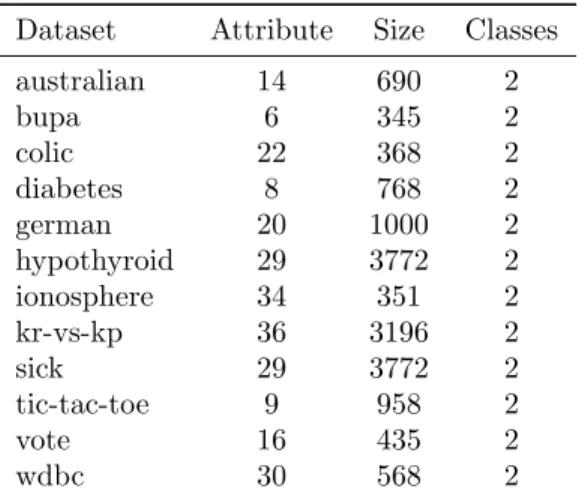
In order to compare the performance of the proposed algorithm with the original tri-training algorithm, we conducted a set of experiments on the 12 datasets from UCI Machine Learning Repository [28]. The properties of datasets are summarized in Table 1.
For each dataset, we use 25% samples in the dataset as test data, and the rest 75% are for training. As we are testing the SSL algorithm, not all training data are used with labels, although all data are labeled. We artificially set 20% of the data as labeled and the rest 80% as unlabeled. For example, assuming we have a dataset containing 1000 instances, 250 instances are used as test data, 750 instances are used as training data, among which 150 out of 750 instances are considered as labeled and the rest 600 out of 750 instances are treated as unlabeled. The selection of training and test sets is randomized while preserving the original ratio of positive and negative classes in all sets.
Table 1: Dataset characteristics
Dataset Attribute Size Classes
australian 14 690 2 bupa 6 345 2 colic 22 368 2 diabetes 8 768 2 german 20 1000 2 hypothyroid 29 3772 2 ionosphere 34 351 2 kr-vs-kp 36 3196 2 sick 29 3772 2 tic-tac-toe 9 958 2 vote 16 435 2 wdbc 30 568 2
The proposed algorithm is implemented on Java SE 8 (revision 1.8.0 45), using Weka [29] data mining library version 3.7.12 for base classification algo-rithms.
We use three methods to create different views from the same training data, namely, use of different learning models, use differently manipulated features, or a combination of the above.
For the different learning models, we use random tree [30], Naive Bayes classifier [31], J4.8 decision trees [32] and the kNN [33] with k = 5 as three different learning models.
The methods of manipulated features include all original features, subsets of features and transformed features. We simply use principal component analysis (PCA) for transforming the features and a variant of the competitive swarm optimizer (CSO) [34], which has been shown to work well for large scale opti-mization to select optimized feature subsets.
We use the average error rates of n-fold cross validation (with n = 3) on labeled data as the fitness function of the CSO to reduce the risk of overfitting in selecting feature subsets. Other parameters in the CSO algorithms are set as follows. The population size is 30, the max number of iterations is 100,φis 0.1. In the first iteration, particles are randomly initialized between [0,1] and the threshold parameterλis 0.5. The variance covered in PCA transformation is set to 0.95. Finally,σin the Multi-Train algorithm is set to 0.5.
To make the comparisons as fair as possible, we apply feature manipulation prior to building the SSL base learners. In this way, we are able to directly compare the classification error rates of single classifiers, tri-training classifiers and the Multi-Train algorithm.
Each algorithm is run for 25 times independently, and the average results are presented and discussed in the following section.
4.2. Empirical Results
We break down the comparison into three parts. In the first part, we compare ensembles whose base learners use features generated using the same feature manipulation method, while in the second part, the classifier models are the same. The last part of the comparison compares Multi-Train ensembles using a combination of different features and different models.
4.2.1. Comparisons of ensembles with different classifier models
We employ three different feature manipulation methods in our tests. The first comparisons aim to demonstrate the benefits of using different classifier models. Therefore, we use a fixed feature manipulation method but different classifier models for comparisons.
In the tables, “MT” denotes Multi-Train and “TT” means tri-training algo-rithms respectively. If there are no prefixs, then these are supervised learning algorithms. “CSO”, “PCA”, and “NONE” indicate the feature manipulation methods, which are CSO-based feature selection, PCA-based feature transfor-mation (dimension reduction), and the original features, respectively. In addi-tion, “RT”, “NB”, “J48”, and “kNN” denote the learning algorithms, which are random trees, Naive Bayes classifiers, J4.8 decision trees and thekNN algorithm, respectively. All results are shown in Tables 2, 3 and 4, respectively.
The first column in each table lists the result of Multi-Train containing four base learners, with each member being trained using features obtained from the same feature manipulation method, while different classifier models are adopted
Table 2: The classification error rate of Multi-Train, tri-training and single classifier with features selected by the CSO-based algorithm
Dataset MT-CSO TT-CSO-RT TT-CSO-NB TT-CSO-J48 TT-CSO-kNN CSO-RT CSO-NB CSO-J48 CSO-kNN australian 0.1285 0.1946+ 0.2079+ 0.1759+ 0.1622+ 0.2019+ 0.2083+ 0.1514+ 0.1422+ (0.0181) (0.0504) (0.0595) (0.0424) (0.0376) (0.0445) (0.0630) (0.0334) (0.0221) bupa 0.3586 0.4199+ 0.4556+ 0.4080+ 0.3996+ 0.4019+ 0.4598+ 0.3954+ 0.3667= (0.0613) (0.0636) (0.0658) (0.0592) (0.0660) (0.0666) (0.0625) (0.0647) (0.0512) colic 0.1493 0.2326+ 0.2072+ 0.2101+ 0.1924+ 0.2424+ 0.1899+ 0.1986+ 0.1768+ (0.0319) (0.0679) (0.0526) (0.0637) (0.0429) (0.0785) (0.0461) (0.0471) (0.0423) diabetes 0.2446 0.3111+ 0.2589+ 0.3023+ 0.2950+ 0.3241+ 0.2486= 0.2917+ 0.2778+ (0.0315) (0.0409) (0.0297) (0.0425) (0.0388) (0.0355) (0.0256) (0.0562) (0.0384) german 0.2729 0.3288+ 0.2956+ 0.3319+ 0.3151+ 0.3417+ 0.2864+ 0.3219+ 0.2988+ (0.0251) (0.0312) (0.0283) (0.0322) (0.0334) (0.0358) (0.0243) (0.0373) (0.0262) hypothyroid 0.0339 0.0423+ 0.0543+ 0.0358= 0.0437+ 0.0447+ 0.0554+0.0331= 0.0410+ (0.0170) (0.0235) (0.0114) (0.0192) (0.0182) (0.0292) (0.0112) (0.0190) (0.0177) ionosphere 0.0996 0.1742+ 0.1735+ 0.1739+ 0.1985+ 0.1773+ 0.1610+ 0.1595+ 0.1837+ (0.0430) (0.0682) (0.0629) (0.0672) (0.0616) (0.0599) (0.0696) (0.0586) (0.0436) kr-vs-kp 0.0436 0.0525+ 0.1065+ 0.0475= 0.0786+ 0.0563+ 0.0993+ 0.0451= 0.0761+ (0.0107) (0.0140) (0.0295) (0.0123) (0.0184) (0.0142) (0.0282) (0.0124) (0.0179) sick 0.0243 0.0360+ 0.0562+ 0.0285= 0.0326+ 0.0391+ 0.0591+ 0.0263= 0.0292+ (0.0063) (0.0109) (0.0260) (0.0094) (0.0076) (0.0096) (0.0248) (0.0080) (0.0056) tic-tac-toe 0.2353 0.2987+ 0.3106+ 0.3003+ 0.2671+ 0.2892+ 0.2901+ 0.2979+ 0.2425= (0.0286) (0.0400) (0.0299) (0.0453) (0.0344) (0.0447) (0.0269) (0.0384) (0.0352) vote 0.0343 0.0554+ 0.0523+ 0.0520+ 0.0596+ 0.0532+ 0.0489+ 0.0526+ 0.0529+ (0.0154) (0.0284) (0.0217) (0.0330) (0.0269) (0.0254) (0.0245) (0.0242) (0.0250) wdbc 0.0387 0.0798+ 0.0587+ 0.0772+ 0.0545+ 0.0892+ 0.0528+ 0.0829+ 0.0469+ (0.0149) (0.0305) (0.0175) (0.0300) (0.0181) (0.0331) (0.0166) (0.0324) (0.0152) avg 0.1386 0.1855 0.1864 0.1786 0.1749 0.1884 0.1800 0.1714 0.1612 win/lose/tie 12/0/0 12/0/0 9/0/3 12/0/0 12/0/0 11/0/1 9/0/3 10/0/2
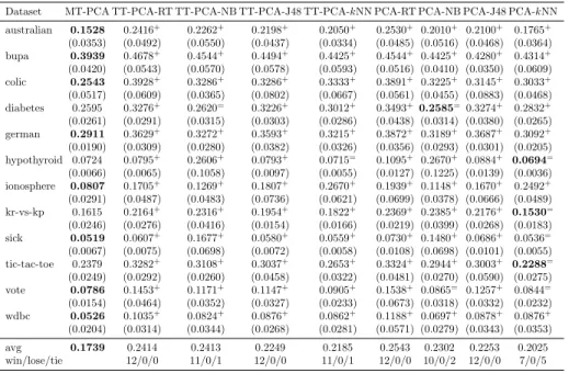
Table 3: The classification error rate of Multi-Train, tri-training and single classifier with features transformed by PCA
Dataset MT-PCA TT-PCA-RT TT-PCA-NB TT-PCA-J48 TT-PCA-kNN PCA-RT PCA-NB PCA-J48 PCA-kNN australian 0.1528 0.2416+ 0.2262+ 0.2198+ 0.2050+ 0.2530+ 0.2010+ 0.2100+ 0.1765+ (0.0353) (0.0492) (0.0550) (0.0437) (0.0334) (0.0485) (0.0516) (0.0468) (0.0364) bupa 0.3939 0.4678+ 0.4544+ 0.4494+ 0.4425+ 0.4544+ 0.4425+ 0.4280+ 0.4314+ (0.0420) (0.0543) (0.0570) (0.0578) (0.0593) (0.0516) (0.0410) (0.0350) (0.0609) colic 0.2543 0.3928+ 0.3286+ 0.3286+ 0.3333+ 0.3891+ 0.3225+ 0.3145+ 0.3033+ (0.0517) (0.0609) (0.0365) (0.0802) (0.0667) (0.0561) (0.0455) (0.0883) (0.0468) diabetes 0.2595 0.3276+ 0.2620= 0.3226+ 0.3012+ 0.3493+0.2585= 0.3274+ 0.2832+ (0.0261) (0.0291) (0.0315) (0.0303) (0.0286) (0.0438) (0.0314) (0.0380) (0.0265) german 0.2911 0.3629+ 0.3272+ 0.3593+ 0.3215+ 0.3872+ 0.3189+ 0.3687+ 0.3092+ (0.0190) (0.0309) (0.0280) (0.0382) (0.0326) (0.0356) (0.0293) (0.0301) (0.0205) hypothyroid 0.0724 0.0795+ 0.2606+ 0.0793+ 0.0715= 0.1095+ 0.2670+ 0.0884+ 0.0694= (0.0066) (0.0065) (0.1058) (0.0097) (0.0055) (0.0127) (0.1225) (0.0139) (0.0036) ionosphere 0.0807 0.1705+ 0.1269+ 0.1807+ 0.2670+ 0.1939+ 0.1148+ 0.1670+ 0.2492+ (0.0291) (0.0487) (0.0483) (0.0736) (0.0621) (0.0699) (0.0378) (0.0666) (0.0489) kr-vs-kp 0.1615 0.2164+ 0.2316+ 0.1954+ 0.1822+ 0.2369+ 0.2385+ 0.2176+ 0.1530= (0.0246) (0.0276) (0.0416) (0.0154) (0.0166) (0.0219) (0.0399) (0.0268) (0.0183) sick 0.0519 0.0607+ 0.1677+ 0.0580+ 0.0559+ 0.0730+ 0.1480+ 0.0686+ 0.0536= (0.0067) (0.0075) (0.0698) (0.0072) (0.0058) (0.0108) (0.0698) (0.0101) (0.0055) tic-tac-toe 0.2379 0.3282+ 0.3108+ 0.3037+ 0.2653+ 0.3324+ 0.2944+ 0.3003+ 0.2288= (0.0249) (0.0292) (0.0260) (0.0458) (0.0322) (0.0481) (0.0270) (0.0590) (0.0275) vote 0.0786 0.1453+ 0.1171+ 0.1147+ 0.0905+ 0.1538+ 0.0865= 0.1257+ 0.0844= (0.0154) (0.0464) (0.0352) (0.0327) (0.0233) (0.0673) (0.0318) (0.0332) (0.0232) wdbc 0.0526 0.1035+ 0.0824+ 0.0876+ 0.0862+ 0.1188+ 0.0697+ 0.0878+ 0.0876+ (0.0204) (0.0314) (0.0344) (0.0268) (0.0281) (0.0571) (0.0279) (0.0343) (0.0353) avg 0.1739 0.2414 0.2413 0.2249 0.2185 0.2543 0.2302 0.2253 0.2025 win/lose/tie 12/0/0 11/0/1 12/0/0 11/0/1 12/0/0 10/0/2 12/0/0 7/0/5
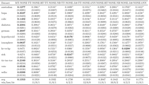
Table 4: The classification error rate of Multi-Train, tri-training and single classifier with all original features
Dataset MT-NONE TT-NONE-RT TT-NONE-NB TT-NONE-J48 TT-NONE-kNN NONE-RT NONE-NB NONE-J48 NONE-kNN australian 0.1277 0.1961+ 0.2110+ 0.1699+ 0.1551+ 0.2291+ 0.2081+ 0.1703+ 0.1412+ (0.0205) (0.0455) (0.0387) (0.0368) (0.0275) (0.0462) (0.0316) (0.0471) (0.0250) bupa 0.3337 0.4008+ 0.4368+ 0.3969+ 0.4299+ 0.3847+ 0.4291+ 0.3893+ 0.4138+ (0.0423) (0.0629) (0.0518) (0.0623) (0.0564) (0.0650) (0.0531) (0.0568) (0.0549) colic 0.1402 0.2804+ 0.2257+ 0.2130+ 0.2156+ 0.3134+ 0.2112+ 0.2047+ 0.1862+ (0.0332) (0.0658) (0.0475) (0.0662) (0.0347) (0.0699) (0.0445) (0.0625) (0.0343) diabetes 0.2394 0.2984+ 0.2651+ 0.3071+ 0.2946+ 0.3349+ 0.2502+ 0.2983+ 0.2766+ (0.0201) (0.0357) (0.0279) (0.0382) (0.0314) (0.0393) (0.0308) (0.0438) (0.0292) german 0.2687 0.3341+ 0.2916+ 0.3376+ 0.3211+ 0.3552+ 0.2737= 0.3359+ 0.3091+ (0.0209) (0.0293) (0.0284) (0.0341) (0.0212) (0.0288) (0.0280) (0.0308) (0.0238) hypothyroid 0.0454 0.0423= 0.0454= 0.0176− 0.0806+ 0.0452= 0.0459= 0.0179− 0.0772+ (0.0088) (0.0129) (0.0092) (0.0065) (0.0071) (0.0193) (0.0095) (0.0069) (0.0047) ionosphere 0.0837 0.1621+ 0.1640+ 0.1545+ 0.2383+ 0.1761+ 0.1568+ 0.1477+ 0.1970+ (0.0356) (0.0513) (0.0551) (0.0557) (0.0666) (0.0516) (0.0562) (0.0662) (0.0577) kr-vs-kp 0.0475 0.0924+ 0.1521+ 0.0366− 0.1358+ 0.0956+ 0.1364+ 0.0298− 0.1224+ (0.0107) (0.0284) (0.0253) (0.0138) (0.0180) (0.0359) (0.0211) (0.0082) (0.0146) sick 0.0274 0.0403+ 0.0759+ 0.0247= 0.0527+ 0.0432+ 0.0802+ 0.0251= 0.0526+ (0.0054) (0.0100) (0.0221) (0.0066) (0.0075) (0.0132) (0.0225) (0.0065) (0.0068) tic-tac-toe 0.2160 0.3018+ 0.3188+ 0.2853+ 0.2551+ 0.3089+ 0.2954+ 0.2883+ 0.2390+ (0.0218) (0.0358) (0.0287) (0.0351) (0.0265) (0.0387) (0.0255) (0.0431) (0.0255) vote 0.0538 0.0841+ 0.0792+ 0.0581= 0.0728+ 0.0844+ 0.0768+ 0.0615= 0.0682+ (0.0138) (0.0408) (0.0168) (0.0329) (0.0194) (0.0330) (0.0198) (0.0279) (0.0198) wdbc 0.0399 0.0690+ 0.0523+ 0.0744+ 0.0507+ 0.0852+ 0.0469+ 0.0833+ 0.0453= (0.0116) (0.0221) (0.0149) (0.0284) (0.0218) (0.0390) (0.0135) (0.0341) (0.0198) avg 0.1353 0.1918 0.1932 0.1730 0.1919 0.2047 0.1842 0.1710 0.1774 win/lose/tie 11/0/1 11/0/1 8/2/2 12/0/0 11/0/1 10/0/2 8/2/2 11/0/1
for base learners. The following four columns present results of four settings of the tri-training algorithm. Each setting uses features pre-manipulated the same as the Multi-Train algorithm and classifier models as noted. Other settings are the same as suggested in the tri-training algorithm. The last four columns show the results from the single classifier with feature being manipulated as in the Multi-Train algorithm, and the classifier models as well.
We used the Wilcoxon rank sum test to verify the significance of the im-provement of the proposed algorithm, symbol ‘+’ denotes the particular setup is significantly outperformed by Multi-Train, while ‘-’ denotes the particular setup is significantly better than Multi-Train, and finally ‘=’ denotes that there is no statistically significant difference between the results obtained by Multi-Train and the particular setup. Those results are also concluded as “win/lose/tie” at the bottom of each table.
Our results shown in Tables 2, 3 and 4 demonstrate that the proposed al-gorithm is statistically outperformed by only in four out of the 288 different settings, which is when the J48 decision tree is used as the learning model. By taking a closer look, we find that the J48 decision tree alone generalizes much better than other learning models on these particular datasets, while other mod-els produce much large errors on the same datasets. It is thus understandable that other models can degrade the overall performance of the ensembles as they give significant more errors. Thus, the proposed algorithm performed worse than setups using J48 decision tree alone. However, as none of these classifier models constantly outperform others, we can still conclude that the proposed algorithm is very competitive with others.
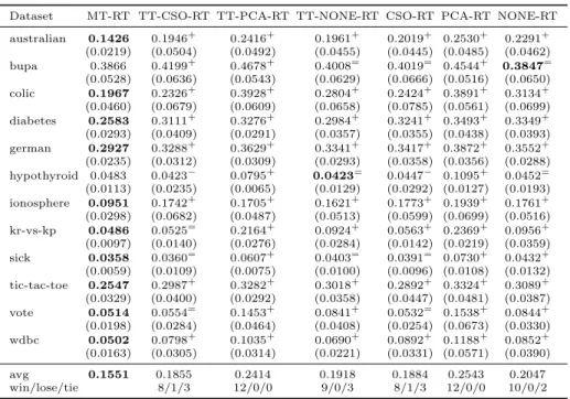
4.2.2. Comparisons of ensembles using different feature manipulation methods Table 5: The classification error rate of Multi-Train, tri-training and single classifier with random tree classifier model
Dataset MT-RT TT-CSO-RT TT-PCA-RT TT-NONE-RT CSO-RT PCA-RT NONE-RT
australian 0.1426 0.1946+ 0.2416+ 0.1961+ 0.2019+ 0.2530+ 0.2291+ (0.0219) (0.0504) (0.0492) (0.0455) (0.0445) (0.0485) (0.0462) bupa 0.3866 0.4199+ 0.4678+ 0.4008= 0.4019= 0.4544+ 0.3847= (0.0528) (0.0636) (0.0543) (0.0629) (0.0666) (0.0516) (0.0650) colic 0.1967 0.2326+ 0.3928+ 0.2804+ 0.2424+ 0.3891+ 0.3134+ (0.0460) (0.0679) (0.0609) (0.0658) (0.0785) (0.0561) (0.0699) diabetes 0.2583 0.3111+ 0.3276+ 0.2984+ 0.3241+ 0.3493+ 0.3349+ (0.0293) (0.0409) (0.0291) (0.0357) (0.0355) (0.0438) (0.0393) german 0.2927 0.3288+ 0.3629+ 0.3341+ 0.3417+ 0.3872+ 0.3552+ (0.0235) (0.0312) (0.0309) (0.0293) (0.0358) (0.0356) (0.0288) hypothyroid 0.0483 0.0423− 0.0795+ 0.0423= 0.0447− 0.1095+ 0.0452= (0.0113) (0.0235) (0.0065) (0.0129) (0.0292) (0.0127) (0.0193) ionosphere 0.0951 0.1742+ 0.1705+ 0.1621+ 0.1773+ 0.1939+ 0.1761+ (0.0298) (0.0682) (0.0487) (0.0513) (0.0599) (0.0699) (0.0516) kr-vs-kp 0.0486 0.0525= 0.2164+ 0.0924+ 0.0563+ 0.2369+ 0.0956+ (0.0097) (0.0140) (0.0276) (0.0284) (0.0142) (0.0219) (0.0359) sick 0.0358 0.0360= 0.0607+ 0.0403= 0.0391= 0.0730+ 0.0432+ (0.0059) (0.0109) (0.0075) (0.0100) (0.0096) (0.0108) (0.0132) tic-tac-toe 0.2547 0.2987+ 0.3282+ 0.3018+ 0.2892+ 0.3324+ 0.3089+ (0.0329) (0.0400) (0.0292) (0.0358) (0.0447) (0.0481) (0.0387) vote 0.0514 0.0554= 0.1453+ 0.0841+ 0.0532= 0.1538+ 0.0844+ (0.0198) (0.0284) (0.0464) (0.0408) (0.0254) (0.0673) (0.0330) wdbc 0.0502 0.0798+ 0.1035+ 0.0690+ 0.0892+ 0.1188+ 0.0852+ (0.0163) (0.0305) (0.0314) (0.0221) (0.0331) (0.0571) (0.0390) avg 0.1551 0.1855 0.2414 0.1918 0.1884 0.2543 0.2047 win/lose/tie 8/1/3 12/0/0 9/0/3 8/1/3 12/0/0 10/0/2
As the original co-training algorithm learns two classifier models from two different “views” of data, and the “views” are actually different sets of features, it might be of interest to examine the influence of different feature manipulation methods on the performance.
Tables 5, 6, 7, and 8 show the comparative results obtained by ensembles with different feature manipulation methods. The results show that using dif-ferent feature manipulation methods can also help enhance the performance of the proposed method. The proposed algorithm is statistically outperformed by others only in six out of 288 compared settings.
The results in this set of the comparison confirmed the conclusions drawn from the first set of the comparisons.
4.2.3. Comparison of heterogeneous ensembles
In the previous comparisons, we use different classifier models or different feature manipulation methods to create diversity among the base learners. The results show that the proposed Multi-Train algorithm has achieved statically better performance than the tri-training algorithm and non-SSL methods. We are interested in investigating whether a larger ensemble containing more base learners is able to further improve the generalization capability.
The last set of experiments to be made in this work is to compare ensem-bles generated using a combination of the settings used in the first two sets of
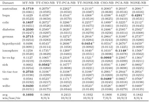
Table 6: The classification error rate of Multi-Train, tri-training and single classifier with Naive Bayes classifier model
Dataset MT-NB TT-CSO-NB TT-PCA-NB TT-NONE-NB CSO-NB PCA-NB NONE-NB
australian 0.1719 0.2079+ 0.2262+ 0.2110+ 0.2083+ 0.2010+ 0.2081+ (0.0361) (0.0595) (0.0550) (0.0387) (0.0630) (0.0516) (0.0316) bupa 0.4429 0.4556= 0.4544= 0.4368= 0.4598= 0.4425= 0.4291= (0.0523) (0.0658) (0.0570) (0.0518) (0.0625) (0.0410) (0.0531) colic 0.1837 0.2072+ 0.3286+ 0.2257+ 0.1899= 0.3225+ 0.2112+ (0.0451) (0.0526) (0.0365) (0.0475) (0.0461) (0.0455) (0.0445) diabetes 0.2330 0.2589+ 0.2620+ 0.2651+ 0.2486+ 0.2585+ 0.2502+ (0.0247) (0.0297) (0.0315) (0.0279) (0.0256) (0.0314) (0.0308) german 0.2715 0.2956+ 0.3272+ 0.2916+ 0.2864+ 0.3189+ 0.2737= (0.0254) (0.0283) (0.0280) (0.0284) (0.0243) (0.0293) (0.0280) hypothyroid 0.0496 0.0543+ 0.2606+ 0.0454= 0.0554+ 0.2670+ 0.0459= (0.0091) (0.0114) (0.1058) (0.0092) (0.0112) (0.1225) (0.0095) ionosphere 0.1258 0.1735+ 0.1269= 0.1640+ 0.1610+ 0.1148= 0.1568+ (0.0520) (0.0629) (0.0483) (0.0551) (0.0696) (0.0378) (0.0562) kr-vs-kp 0.1127 0.1065= 0.2316+ 0.1521+ 0.0993= 0.2385+ 0.1364+ (0.0219) (0.0295) (0.0416) (0.0253) (0.0282) (0.0399) (0.0211) sick 0.0662 0.0562= 0.1677+ 0.0759+ 0.0591= 0.1480+ 0.0802+ (0.0254) (0.0260) (0.0698) (0.0221) (0.0248) (0.0698) (0.0225) tic-tac-toe 0.2733 0.3106+ 0.3108+ 0.3188+ 0.2901+ 0.2944+ 0.2954+ (0.0198) (0.0299) (0.0260) (0.0287) (0.0269) (0.0270) (0.0255) vote 0.0584 0.0523= 0.1171+ 0.0792+ 0.0489= 0.0865+ 0.0768+ (0.0192) (0.0217) (0.0352) (0.0168) (0.0245) (0.0318) (0.0198) wdbc 0.0430 0.0587+ 0.0824+ 0.0523+ 0.0528+ 0.0697+ 0.0469= (0.0151) (0.0175) (0.0344) (0.0149) (0.0166) (0.0279) (0.0135) avg 0.1693 0.1864 0.2413 0.1932 0.1800 0.2302 0.1842 win/lose/tie 8/0/4 10/0/2 10/0/2 7/0/5 10/0/2 8/0/4
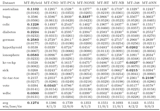
empirical studies. As shown in Table 9, eight settings are considered in this comparison, including MT-Hybrid, MT-CSO, MT-PCA, MT-NONE, MT-RT, MT-NB, MT-J48, and MT-kNN. The differences among the settings lie mainly in the base learners as well as the features the base learners use for creating diversity. MT-Hybrid creates diversity by using a combination of three different feature manipulation methods and four different classifier models, resulting in 12 different base learners. MT-CSO, MT-PCA, and MT-NONE have the same settings as those in Section 4.2.1, which create diversity by using four different classifier models. Therefore, the number of base learners is four. Finally, MT-RT, MT-NB, MT-J48, and MT-kNN are settings used in Section 4.2.2, which create diversity by using three different feature manipulation methods. The number of base learners is thus three.
The results show that MT-Hybrid has the lowest average error rate. The statistical tests also confirm that MT-hybrid outperforms other methods, ex-cept for one setting using MT-CSO and MT-NONE, and two settings using MT-J48. These findings re-confirm that heterogeneous ensembles have better generalization ability.
5. Conclusion
We propose a new ensemble based semi-supervised learning algorithm in this paper, namely Multi-Train. By comparing it with the tri-training
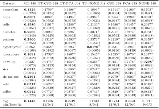
algo-Table 7: The classification error rate of Multi-Train, tri-training and single classifier with J4.8 decision tree classifier model
Dataset MT-J48 TT-CSO-J48 TT-PCA-J48 TT-NONE-J48 CSO-J48 PCA-J48 NONE-J48 australian 0.1329 0.1759+ 0.2198+ 0.1699+ 0.1514+ 0.2100+ 0.1703+ (0.0229) (0.0424) (0.0437) (0.0368) (0.0334) (0.0468) (0.0471) bupa 0.3567 0.4080+ 0.4494+ 0.3969+ 0.3954+ 0.4280+ 0.3893+ (0.0526) (0.0592) (0.0578) (0.0623) (0.0647) (0.0350) (0.0568) colic 0.1580 0.2101+ 0.3286+ 0.2130+ 0.1986+ 0.3145+ 0.2047+ (0.0357) (0.0637) (0.0802) (0.0662) (0.0471) (0.0883) (0.0625) diabetes 0.2566 0.3023+ 0.3226+ 0.3071+ 0.2917+ 0.3274+ 0.2983+ (0.0349) (0.0425) (0.0303) (0.0382) (0.0562) (0.0380) (0.0438) german 0.2960 0.3319+ 0.3593+ 0.3376+ 0.3219+ 0.3687+ 0.3359+ (0.0256) (0.0322) (0.0382) (0.0341) (0.0373) (0.0301) (0.0308) hypothyroid 0.0262 0.0358+ 0.0793+ 0.0176= 0.0331+ 0.0884+ 0.0179= (0.0166) (0.0192) (0.0097) (0.0065) (0.0190) (0.0139) (0.0069) ionosphere 0.1091 0.1739+ 0.1807+ 0.1545+ 0.1595+ 0.1670+ 0.1477+ (0.0348) (0.0672) (0.0736) (0.0557) (0.0586) (0.0666) (0.0662) kr-vs-kp 0.0327 0.0475+ 0.1954+ 0.0366= 0.0451+ 0.2176+ 0.0298= (0.0070) (0.0123) (0.0154) (0.0138) (0.0124) (0.0268) (0.0082) sick 0.0215 0.0285+ 0.0580+ 0.0247= 0.0263+ 0.0686+ 0.0251+ (0.0041) (0.0094) (0.0072) (0.0066) (0.0080) (0.0101) (0.0065) tic-tac-toe 0.2361 0.3003+ 0.3037+ 0.2853+ 0.2979+ 0.3003+ 0.2883+ (0.0304) (0.0453) (0.0458) (0.0351) (0.0384) (0.0590) (0.0431) vote 0.0517 0.0520= 0.1147+ 0.0581= 0.0526= 0.1257+ 0.0615= (0.0225) (0.0330) (0.0327) (0.0329) (0.0242) (0.0332) (0.0279) wdbc 0.0542 0.0772+ 0.0876+ 0.0744+ 0.0829+ 0.0878+ 0.0833+ (0.0228) (0.0300) (0.0268) (0.0284) (0.0324) (0.0343) (0.0341) avg 0.1443 0.1786 0.2249 0.1730 0.1714 0.2253 0.1710 win/lose/tie 11/0/1 12/0/0 8/0/4 11/0/1 12/0/0 9/0/3
Table 8: The classification error rate of Multi-Train, tri-training and single classifier withkNN classifier model
Dataset MT-kNN TT-CSO-kNN TT-PCA-kNN TT-NONE-kNN CSO-kNN PCA-kNN NONE-kNN australian 0.1243 0.1622+ 0.2050+ 0.1551+ 0.1422+ 0.1765+ 0.1412+ (0.0187) (0.0376) (0.0334) (0.0275) (0.0221) (0.0364) (0.0250) bupa 0.3663 0.3996+ 0.4425+ 0.4299+ 0.3667= 0.4314+ 0.4138+ (0.0465) (0.0660) (0.0593) (0.0564) (0.0512) (0.0609) (0.0549) colic 0.1551 0.1924+ 0.3333+ 0.2156+ 0.1768+ 0.3033+ 0.1862+ (0.0307) (0.0429) (0.0667) (0.0347) (0.0423) (0.0468) (0.0343) diabetes 0.2552 0.2950+ 0.3012+ 0.2946+ 0.2778+ 0.2832+ 0.2766+ (0.0270) (0.0388) (0.0286) (0.0314) (0.0384) (0.0265) (0.0292) german 0.2839 0.3151+ 0.3215+ 0.3211+ 0.2988+ 0.3092+ 0.3091+ (0.0211) (0.0334) (0.0326) (0.0212) (0.0262) (0.0205) (0.0238) hypothyroid 0.0649 0.0437− 0.0715+ 0.0806+ 0.0410− 0.0694+ 0.0772+ (0.0034) (0.0182) (0.0055) (0.0071) (0.0177) (0.0036) (0.0047) ionosphere 0.2034 0.1985= 0.2670+ 0.2383+ 0.1837= 0.2492+ 0.1970= (0.0551) (0.0616) (0.0621) (0.0666) (0.0436) (0.0489) (0.0577) kr-vs-kp 0.0663 0.0786+ 0.1822+ 0.1358+ 0.0761+ 0.1530+ 0.1224+ (0.0128) (0.0184) (0.0166) (0.0180) (0.0179) (0.0183) (0.0146) sick 0.0394 0.0326− 0.0559+ 0.0527+ 0.0292− 0.0536+ 0.0526+ (0.0060) (0.0076) (0.0058) (0.0075) (0.0056) (0.0055) (0.0068) tic-tac-toe 0.2108 0.2671+ 0.2653+ 0.2551+ 0.2425+ 0.2288+ 0.2390+ (0.0286) (0.0344) (0.0322) (0.0265) (0.0352) (0.0275) (0.0255) vote 0.0578 0.0596= 0.0905+ 0.0728+ 0.0529= 0.0844+ 0.0682+ (0.0158) (0.0269) (0.0233) (0.0194) (0.0250) (0.0232) (0.0198) wdbc 0.0336 0.0545+ 0.0862+ 0.0507+ 0.0469+ 0.0876+ 0.0453+ (0.0139) (0.0181) (0.0281) (0.0218) (0.0152) (0.0353) (0.0198) avg 0.1551 0.1749 0.2185 0.1919 0.1612 0.2025 0.1774 win/lose/tie 8/2/2 12/0/0 12/0/0 7/2/3 12/0/0 11/0/1
Table 9: The classification error rate of Multi-Train with different heterogeneous base learner sets
Dataset MT-Hybrid MT-CSO MT-PCA MT-NONE MT-RT MT-NB MT-J48 MT-kNN
australian 0.1102 0.1285+ 0.1528+ 0.1277+ 0.1426+ 0.1719+ 0.1329+ 0.1243+ (0.0183) (0.0181) (0.0353) (0.0205) (0.0219) (0.0361) (0.0229) (0.0187) bupa 0.3586 0.3586= 0.3939+ 0.3337= 0.3866+ 0.4429+ 0.3567= 0.3663= (0.0506) (0.0613) (0.0420) (0.0423) (0.0528) (0.0523) (0.0526) (0.0465) colic 0.1228 0.1493+ 0.2543+ 0.1402+ 0.1967+ 0.1837+ 0.1580+ 0.1551+ (0.0266) (0.0319) (0.0517) (0.0332) (0.0460) (0.0451) (0.0357) (0.0307) diabetes 0.2224 0.2446+ 0.2595+ 0.2394+ 0.2583+ 0.2330+ 0.2566+ 0.2552+ (0.0232) (0.0315) (0.0261) (0.0201) (0.0293) (0.0247) (0.0349) (0.0270) german 0.2583 0.2729+ 0.2911+ 0.2687+ 0.2927+ 0.2715+ 0.2960+ 0.2839+ (0.0177) (0.0251) (0.0190) (0.0209) (0.0235) (0.0254) (0.0256) (0.0211) hypothyroid 0.0538 0.0339− 0.0724+ 0.0454− 0.0483= 0.0496= 0.0262− 0.0649+ (0.0067) (0.0170) (0.0066) (0.0088) (0.0113) (0.0091) (0.0166) (0.0034) ionosphere 0.0583 0.0996+ 0.0807+ 0.0837+ 0.0951+ 0.1258+ 0.1091+ 0.2034+ (0.0233) (0.0430) (0.0291) (0.0356) (0.0298) (0.0520) (0.0348) (0.0551) kr-vs-kp 0.0328 0.0436+ 0.1615+ 0.0475+ 0.0486+ 0.1127+ 0.0327= 0.0663+ (0.0082) (0.0107) (0.0246) (0.0107) (0.0097) (0.0219) (0.0070) (0.0128) sick 0.0268 0.0243= 0.0519+ 0.0274= 0.0358+ 0.0662+ 0.0215− 0.0394+ (0.0047) (0.0063) (0.0067) (0.0054) (0.0059) (0.0254) (0.0041) (0.0060) tic-tac-toe 0.2157 0.2353+ 0.2379+ 0.2160= 0.2547+ 0.2733+ 0.2361+ 0.2108= (0.0217) (0.0286) (0.0249) (0.0218) (0.0329) (0.0198) (0.0304) (0.0286) vote 0.0394 0.0343= 0.0786+ 0.0538+ 0.0514+ 0.0584+ 0.0517+ 0.0578+ (0.0141) (0.0154) (0.0154) (0.0138) (0.0198) (0.0192) (0.0225) (0.0158) wdbc 0.0300 0.0387+ 0.0526+ 0.0399+ 0.0502+ 0.0430+ 0.0542+ 0.0336= (0.0131) (0.0149) (0.0204) (0.0116) (0.0163) (0.0151) (0.0228) (0.0139) avg 0.1274 0.1386 0.1739 0.1353 0.1551 0.1693 0.1443 0.1551 win/lose/tie 8/1/3 12/0/0 8/1/3 11/0/1 11/0/1 8/2/2 9/0/3
rithm and non-SSL learning models, we show that the proposed Multi-Train ensemble models outperform the compared algorithms. The better performance can be attributed to the multiple views generated using different models as well as different feature manipulation methods in contrast to the original single-view data. Furthermore, by using ensemble method, the prediction accuracy on the unlabeled data is improved, which therefore is able to reduce the risk of incorrectly labelling the unlabeled data [5, 10]. Our results confirm that the heterogeneous ensembles, which consist of different types of based models and use different features have superior generalization performance.
As shown in some scenarios, one base learner in the Multi-Train performs significantly better or worse than other base learners. It is therefore of interest to assign a larger weight to those good base learners while prune the poor ones, which can potentially further increase the generalization ability of Multi-Train.
References
[1] N. Zeng, Z. Wang, B. Zineddin, Y. Li, M. Du, L. Xiao, X. Liu, T. Young, Image-based quantitative analysis of gold immunochromatographic strip via cellular neural network approach, IEEE Transactions on Medical Imag-ing 33 (5) (2014) 1129–1136. doi:10.1109/TMI.2014.2305394.
pso algorithm for estimating unknown parameters of lateral flow
im-munoassay, Cognitive Computation 8 (2) (2016) 143–152. doi:10.1007/
s12559-016-9396-6.
URLhttp://dx.doi.org/10.1007/s12559-016-9396-6
[3] Y. Lu, N. Zeng, Y. Liu, N. Zhang, A hybrid wavelet neural
net-work and switching particle swarm optimization algorithm for
face direction recognition, Neurocomputing 155 (2015) 219 – 224.
doi:http://dx.doi.org/10.1016/j.neucom.2014.12.026.
URL http://www.sciencedirect.com/science/article/pii/ S0925231214016907
[4] M. Belkin, P. Niyogi, Semi-supervised learning on riemannian manifolds, Machine Learning 56 (1) (2004) 209–239.
[5] A. Blum, S. Chawla, Learning from labeled and unlabeled data using graph mincuts, in: Proceedings of the 18th International Conference on Machine Learning, ICML ’01, Morgan Kaufmann Publishers Inc., San Francisco, CA, USA, 2001, pp. 19–26.
URLhttp://dl.acm.org/citation.cfm?id=645530.757779
[6] D. Zhou, O. Bousquet, T. N. Lal, J. Weston, B. Sch¨olkopf, Learning with local and global consistency, Advances in Neural Information Processing Systems 16 (16) (2004) 321–328.
[7] X. Zhu, Z. Ghahramani, J. Lafferty, Semi-supervised learning using gaus-sian fields and harmonic functions, in: Proceedings of the 20th International Conference on Machine Learning, 2003, pp. 912–919.
[8] A. P. Dempster, N. M. Laird, D. B. Rubin, Maximum Likelihood from Incomplete Data via the EM Algorithm, Journal of the Royal Statistical Society. Series B (Methodological) 39 (1) (1977) 1–38.
[9] D. J. Miller, H. S. Uyar, A Mixture of Experts Classifier with Learning Based on Both Labelled and Unlabelled Data, in: M. C. Mozer, M. I. Jor-dan, T. Petsche (Eds.), Advances in Neural Information Processing Systems 9, MIT Press, 1997, pp. 571–577.
[10] K. Nigam, A. K. Mccallum, S. Thrun, T. Mitchell, Text classification from labeled and unlabeled documents using EM, Machine Learning 39 (2) (2000) 103–134.
[11] B. M. Shahshahani, D. A. Landgrebe, The effect of unlabeled samples in reducing the small sample size problem and mitigating the Hughes phe-nomenon, Geoscience and Remote Sensing, IEEE Transactions on 32 (5) (1994) 1087–1095.
[12] A. Blum, T. Mitchell, Combining labeled and unlabeled data with co-training, in: Proceedings of the 11th Annual Conference on Computational Learning Theory, ACM, 1998, pp. 92–100.
[13] S. A. Goldman, Y. Zhou, Enhancing supervised learning with unlabeled data, in: Proceedings of the 17th International Conference on Machine Learning, ICML ’00, Morgan Kaufmann Publishers Inc., San Francisco, CA, USA, 2000, pp. 327–334.
URLhttp://dl.acm.org/citation.cfm?id=645529.658273
[14] M. Li, Z.-H. Zhou, Improve computer-aided diagnosis with machine learn-ing techniques uslearn-ing undiagnosed samples, Systems, Man and Cybernetics, Part A: Systems and Humans, IEEE Transactions on 37 (6) (2007) 1088– 1098.
[15] S. Yu, B. Krishnapuram, R. o. m. Rosales, R. B. Rao, Bayesian co-training, J. Mach. Learn. Res. 12 (2011) 2649–2680.
[16] Z.-H. Zhou, M. Li, Tri-training: exploiting unlabeled data using three clas-sifiers, IEEE Transactions on Knowledge and Data Engineering 17 (11) (2005) 1529–1541.
[17] Z. H. Zhou, D. C. Zhan, Q. Yang, Semi-supervised learning with very few labeled training examples, in: Proceedings of the National Conference on Artificial Intelligence, Department of Computer Science and Engineering, Hong Kong University of Science and Technology, China, Vancouver, BC, 2007, pp. 675–680.
[18] W. Liu, Z. Wang, X. Liu, N. Zeng, Y. Liu, F. E. Alsaadi, A survey of deep neural network architectures and their applications, Neurocomputing 234
(2017) 11 – 26. doi:http://dx.doi.org/10.1016/j.neucom.2016.12.
038.
URL http://www.sciencedirect.com/science/article/pii/ S0925231216315533
[19] S. Dasgupta, M. L. Littman, D. McAllester, PAC generalization bounds for co-training, in: Advances in Neural Information Processing Systems, 2002, pp. 375–382.
[20] C. Smith, Y. Jin, Evolutionary multi-objective generation of recurrent neural network ensembles for time series prediction, Neurocomputing 143
(2014) 302 – 311. doi:http://dx.doi.org/10.1016/j.neucom.2014.
05.062.
URL http://www.sciencedirect.com/science/article/pii/ S0925231214007279
[21] S. Gu, R. Cheng, Y. Jin, Multi-objective ensemble generation, Wiley Inter-disciplinary Reviews: Data Mining and Knowledge Discovery 5 (5) (2015) 234–245.
[22] M. Claesen, F. D. Smet, J. A. Suykens, B. D. Moor, A
ro-bust ensemble approach to learn from positive and unlabeled data
doi:http://dx.doi.org/10.1016/j.neucom.2014.10.081.
URL http://www.sciencedirect.com/science/article/pii/ S0925231215001174
[23] W. A. Albukhanajer, Y. Jin, J. A. Briffa, Classifier ensembles for image identification using multi-objective Pareto features, NeurocomputingAc-cepted.
[24] W. Shao, X. Tian, Semi-supervised selective ensemble
learn-ing based on distance to model for nonlinear soft sensor
de-velopment, Neurocomputing 222 (2017) 91 – 104. doi:http:
//dx.doi.org/10.1016/j.neucom.2016.10.005.
URL http://www.sciencedirect.com/science/article/pii/ S0925231216311675
[25] W. Xiao, Y. Yang, H. Wang, T. Li, H. Xing, Semi-supervised hierarchical clustering ensemble and its application, Neurocomputing 173, Part 3 (2016)
1362 – 1376. doi:http://dx.doi.org/10.1016/j.neucom.2015.09.009.
URL http://www.sciencedirect.com/science/article/pii/ S092523121501317X
[26] M. Amozegar, K. Khorasani, An ensemble of dynamic neural network iden-tifiers for fault detection and isolation of gas turbine engines, Neural Net-works 76 (2016) 106–121.
[27] B. Seijo-Pardo, I. Porto-Daz, V. Boln-Canedo, A. Alonso-Betanzos,
En-semble feature selection: Homogeneous and heterogeneous approaches,
Knowledge-Based Systems 118 (2017) 124–139.
[28] K. Bache, M. Lichman, UCI machine learning repository (2013). URLhttp://archive.ics.uci.edu/ml
[29] M. Hall, E. Frank, G. Holmes, B. Pfahringer, P. Reutemann, I. H. Witten, The WEKA data mining software: an update, ACM SIGKDD explorations newsletter 11 (1) (2009) 10–18.
[30] Y. Amit, D. Geman, Shape quantization and recognition with randomized trees, Neural Computation 9 (7) (1997) 1545–1588.
[31] K. P. Murphy, Naive bayes classifiers, University of British Columbia. URL http://www.cs.ubc.ca/~murphyk/Teaching/CS340-Fall06/ reading/NB.pdf
[32] I. H. Witten, E. Frank, Data Mining: Practical machine learning tools and techniques, Morgan Kaufmann, 2005.
[33] D. Aha, D. Kibler, M. Albert, Instance-based learning algorithms, Machine Learning 6 (1) (1991) 37–66.
[34] S. Gu, R. Cheng, Y. Jin, Feature selection for high-dimensional classifi-cation using a competitive swarm optimizer, Soft Computing (2016) 1– 12doi:10.1007/s00500-016-2385-6.