Durham Research Online
Deposited in DRO: 27 July 2018
Version of attached le: Accepted Version
Peer-review status of attached le: Peer-reviewed
Citation for published item:
Andreou, P.C. and Kagkadis, A. and Philip, D. and Tuneshev, T. (2018) 'Dierences in options investors' expectations and the cross-section of stock returns.', Journal of banking and nance., 94 . pp. 315-336. Further information on publisher's website:
https://doi.org/10.1016/j.jbankn.2018.07.016 Publisher's copyright statement:
c
2018 This manuscript version is made available under the CC-BY-NC-ND 4.0 license http://creativecommons.org/licenses/by-nc-nd/4.0/
Additional information:
Use policy
The full-text may be used and/or reproduced, and given to third parties in any format or medium, without prior permission or charge, for personal research or study, educational, or not-for-prot purposes provided that:
• a full bibliographic reference is made to the original source • alinkis made to the metadata record in DRO
• the full-text is not changed in any way
The full-text must not be sold in any format or medium without the formal permission of the copyright holders. Please consult thefull DRO policyfor further details.
Durham University Library, Stockton Road, Durham DH1 3LY, United Kingdom Tel : +44 (0)191 334 3042 | Fax : +44 (0)191 334 2971
Differences in Options Investors’ Expectations and the
Cross-Section of Stock Returns
∗Panayiotis C. Andreou†§ Anastasios Kagkadis‡ Dennis Philip§ Ruslan Tuneshev¶
This draft: July 2018
Abstract
We provide strong evidence that the dispersion of individual stock options trading volume across moneynesses (IDISP) contains valuable information about future stock returns. Stocks with high IDISP consistently underperform those with low IDISP by more than 1% per month. In line with the idea that IDISP reflects dispersion in investors’ beliefs, we find that the neg-ative IDISP-return relationship is particularly pronounced around earnings announcements, in high sentiment periods and among stocks that exhibit relatively high short-selling impediments. Moreover, the IDISP effect is highly persistent and robustly distinct from the effects of a large array of previously documented cross-sectional return predictors.
JEL Classification: G10, G11, G12, G14
Keywords: Dispersion of beliefs; Disagreement in options market; Cross-section of stock returns; Equity options; Option trading volume
∗
We would like to thank two anonymous referees, Yakov Amihud, Daniel Andrei, Constantinos Antoniou, Kevin Aretz, Eser Arisoy, Turan Bali, Anurag Banerjee, Jie Cao, Ray Chou, Sudipto Dasgupta, Prosper Dovonon, Ingmar Nolte, Ioannis Papantonis, Piet Sercu, George Skiadopoulos, Viktor Todorov, Paul Whelan, Qi Zhang and seminar and conference participants at Lancaster University, Liverpool University, OptionMetrics Research 2015 Conference, MFS Spring 2016 Conference, EFMA 2016 Meeting, Financial Econometrics and Empirical Asset Pricing 2016 Conference, and CEPR 2017 Spring Symposium in Financial Economics for valuable comments and suggestions. All errors are our own responsibility.
†
Department of Commerce, Finance and Shipping, Cyprus University of Technology, 140, Ayiou Andreou Street, 3603 Lemesos, Cyprus; Email: panayiotis.andreou@cut.ac.cy
‡
Department of Accounting and Finance, Lancaster University Management School, Lancaster, LA1 4YX, UK; Email: a.kagkadis@lancaster.ac.uk
§
Durham University Business School, Durham University, Mill Hill Lane, Durham DH1 3LB, UK; Email: den-nis.philip@durham.ac.uk
¶
School of Economics and Finance, University of St Andrews, The Scores, St Andrews, KY16 9AR, UK; rt65@st-andrews.ac.uk
1
Introduction
The bet-like nature of options’ payoffs combined with their embedded leverage render them an ideal instrument for investors to reflect their expectations about the future direction of the underlying asset price. In this spirit, Bali and Hovakimian (2009), Xing, Zhang and Zhao (2010), Cremers and Weinbaum (2010) and An, Ang, Bali and Cakici (2014), among others, show that various empirical measures extracted from option prices encapsulate valuable information about the cross-section of individual stock returns. Unlike previous studies, this paper focuses on the information content embedded in the trading activity of the options market. In particular, it shows that the dispersion of individual stock options trading volume across different moneyness levels (denoted IDISP) is a strong predictor of the cross-section of expected returns.
We postulate that the dispersion of trading volume across moneynesses can be viewed as a proxy for differences in expectations among investors. This dispersion measurement stems from the trading activity in the stock options market, which is mainly driven by investors’ directional expectations about the future price of the underlying asset (Lakonishok, Lee, Pearson and Poteshman, 2007). In this spirit, studies such as those of Pan and Poteshman (2006) and Johnson and So (2012) rely on measures of stock options trading activity as the source of information to capture investors’ beliefs. The options dispersion measure can be motivated in a stylized framework of optimal trad-ing behavior that maximizes investors’ expected utility. Intuitively, this framework presumes that investors who speculate based on their directional expectations about the future stock price choose to trade at the moneyness level that best fulfills their optimistic or pessimistic views. Within this framework, we demonstrate that the optimal moneyness for an investor is proportional to her level of optimism or pessimism. Thus, a more optimistic investor chooses to buy calls or sell puts of a higher strike price, whilst a more pessimistic investor chooses to buy puts or sell calls of a lower strike price. Therefore, high differences of opinion should be associated with high dispersion of volume traded across a large range of strike prices, implying that investors share rather divergent beliefs. Likewise, low differences of opinion should be associated with low dispersion of volume traded at a few adjacent strike prices, implying that investors share rather homogeneous beliefs.
Compared to previously proposed measures, which are based on either the predictions of professional forecasters, investors’ portfolio holdings or stock trading volume, the suggested IDISP measure ex-hibits several advantageous properties.1 First, unlike survey-type proxies, which represent only a restricted subset of opinions, our measure emerges directly from transactions in the options market, which provides a perfect venue for a massive pool of investors to explicitly express their opinions. Second, most of the divergence proxies based on forecasts are influenced by behavioral biases and agency issues between firms and investments banks (see, for example, Trueman, 1994; Dechow, Hutton and Sloan, 2000; Cen, Hilary and Wei, 2013), and are mainly related to earnings or other corporate information. By contrast, our IDISP measure is unlikely to be affected by such biases and directly relates to future stock price movements. Third, unlike dispersion proxies that rely on portfolio holdings data or aggregate volume, our measure can equally incorporate different levels of both optimistic and pessimistic expectations, since the options market is less likely to be influenced by the short-sale constraints present in the equity market (Lakonishok, Lee, Pearson and Potesh-man, 2007). Finally, in comparison to forecasts that are typically released monthly or quarterly, our measure is easily computable at any frequency and can provide investors with direct access to the information about the belief dispersion level for any optioned stock at any time.2
Our empirical results show that high IDISP stocks earn substantially lower returns than low IDISP stocks. In particular, a portfolio-level analysis indicates that stocks sorted into the highest IDISP decile consistently underperform stocks in the lowest IDISP decile, by about 1.5% per month for equal- as well as value-weighted returns. After adjusting for the Carhart (1997) and the Pastor and Stambaugh (2003) factors, the equal-weighted (value-weighted) alpha of a strategy that buys
1Diether, Malloy and Scherbina (2002), Park (2005), Anderson, Ghysels and Juergens (2009), Yu (2011) and Carlin, Longstaff and Matoba (2014) utilize the dispersion in the opinions of professional forecasters. Chen, Hong and Stein (2002), Goetzmann and Massa (2005) and Jiang and Sun (2014) create dispersion proxies using investor portfolio holdings. Garfinkel and Sokobin (2006) and Garfinkel (2009) measure dispersion in beliefs via the trading volume that is not attributable to liquidity or informedness effects, while Sarkar and Schwartz (2009) compute a sidedness measure based on buyer- and seller-initiated trades.
2
In a recent study that appears subsequent to the first draft of this paper, Fournier, Goyenko and Grass (2017) also construct a disagreement proxy from the options trading activity. There are two key differences between the two measures. First, their measure stems from a distinction between optimistic and pessimistic trades, while our measure also distinguishes different degrees of optimism or pessimism. Second, the construction of their measure requires the usage of proprietary signed volume data, while our measure can be constructed either by unsigned or signed volume data and we show that the two constructions of our measure exhibit very similar information content. It is important to note that both studies document negative predictability of options investors’ disagreement for the cross-section of stock returns.
high IDISP stocks and sells low IDISP stocks remains economically substantial and statistically significant, earning -1.54% (-1.59%) per month, with associated t-statistics of -4.88 (-4.23). Due to the fact that our sample consists of stocks for which an options market exists, it is by construction tilted towards relatively big, more liquid and more investable stocks. However, a profitable long-short strategy would also require IDISP to be a persistent stock characteristic, in order to ensure low rebalancing and hence low transaction costs. In light of this, we demonstrate that high IDISP stocks in one month remain high in the subsequent month, with a 56% probability.3 Furthermore, the persistence of IDISP as a stock characteristic implies that the return predictability might be significant even at long horizons. Consistent with this expectation, we show that the risk-adjusted return of a strategy that buys high IDISP stocks and sells low IDISP stocks remains economically and statistically significant even when considering a 12-month holding period.4 Finally, we find that the information content of IDISP for future stock returns is not subsumed by more than twenty previously documented predictive characteristics such as idiosyncratic volatility, maximum return, default risk, risk-neutral skewness, and volatility of volatility.
As discussed above, our theoretical framework describes an environment where investors express their directional views via naked option positions. However, it can be easily extended to cases where investors rely on the put-call parity to create synthetic positions. For example, an optimistic investor can replicate an out-of-the-money (OTM) call purchase or an in-the-money (ITM) put sale by purchasing a matched-strike ITM put or selling a matched strike OTM call respectively. The main prediction of our framework – that the optimal moneyness level for an investor is proportional to her level of optimism or pessimism – holds in the case of synthetic positions as well. On the other hand, such complicated put-call parity strategies might be relatively difficult for investors to implement. Therefore, we examine the predictability of an IDISP measure that is estimated using only the trades that are easily implementable and are clearly associated with investors’ expecta-tions, i.e. the buy-side volume of OTM options and the sell-side volume of ITM options. The
3
Note that the trading strategy that exploits the information content of IDISP requires short-selling the high IDISP stocks and hence the average investor would typically find it difficult to implement. However, the strategy would be easily implementable by certain institutional investors, such as hedge funds, who face low short-sale constraints. For example, recent literature emphasizes that some institutional investors do short-sell overpriced stocks regularly and realize significant gains (Boehmer, Jones, and Zhang, 2008; Diether, Lee and Werner, 2009).
4
The dispersion in options investors’ beliefs is also shown to be a strong negative predictor of the equity premium across various horizons (see Andreou, Kagkadis, Maio and Philip, 2018).
underperformance of high IDISP stocks relative to low IDISP stocks is reconfirmed in this case, even though this analysis covers a smaller sample period since the respective signed volume data are first recorded in 2005. For example, the equal- and value-weighted five-factor alphas of a high minus low IDISP portfolio are both about -1.7% per month and highly significant at the 1% level.
The observed negative predictability of IDISP for the cross-section of stock returns implies that high IDISP firms tend to be overpriced and hence investors earn, on average, a negative risk pre-mium when holding such stocks. This result is in line with the findings of several other studies (e.g. Diether, Malloy and Scherbina, 2002; Chen, Hong and Stein, 2002; Goetzmann and Massa, 2005; Boehme, Danielsen and Sorescu, 2006) which show that various proxies for disagreement fore-cast negative individual stock returns. The well-documented negative relation between dispersion in beliefs and future stock returns can be explained in the context of the theoretical mechanism described by Miller (1977). In particular, Miller (1977) suggests that binding short-sale constraints prevents pessimistic agents from revealing their negative valuations and hence the equilibrium price is determined only by the most optimistic of the investors. Therefore, in the presence of short-sale constraints, a high dispersion in beliefs leads to an upward bias in the stock price and hence high differences of opinion are associated with negative future returns.
We further explore the economic nature of the documented relation between IDISP and future stock returns. First, Miller’s (1977) theory requires that the predictability of any dispersion in beliefs proxy be stronger among stocks that exhibit higher short-sale costs and limits to arbitrage. Intuitively, high short-sale costs allow the overpricing to be generated, while high limits to arbi-trage prevent an instant correction. In line with the notion that IDISP captures investors’ diverse beliefs, we find that its predictability is mostly associated with those stocks in our sample that exhibit lower levels of residual institutional ownership (proxying for higher short-sale costs) and with stocks that have relatively small market capitalization, low liquidity and high idiosyncratic volatility (proxying for higher limits to arbitrage). Second, the relation between dispersion in be-liefs and returns is expected to be very strong around earnings announcements. This is because the pre-announcement period provides fertile grounds for investors with diverse views to speculate on the outcome, and hence the overpricing related to disagreement and the subsequent correction that
comes when new information is released in the market should be particularly pronounced (Berk-man, Dimitrov, Jain, Koch and Tice, 2009). Our results demonstrate a very strong IDISP effect around earnings announcements, which is consistent with the idea that IDISP behaves as an ef-fective proxy for dispersion in investors’ beliefs. Finally, the effect of dispersion in beliefs on asset prices is expected to be mainly associated with relatively optimistic periods. This is because the overpricing generated by disagreement in the presence of short-sales constraints is more severe when the optimistic investors who end up holding the stock are excessively optimistic (Stambaugh, Yu and Yuan, 2012). In line with the interpretation of IDISP as a proxy for dispersion in beliefs, we show that the predictability of IDISP is mainly driven by relatively optimistic periods.
In summary, this paper creates a novel option-implied firm-level disagreement proxy and shows that it is a strong and robust negative predictor of future stock returns. In this respect, it contributes to an existing literature that develops various disagreement proxies and examines the implications of heterogeneity in beliefs for asset prices (see, for example, Diether, Malloy and Scherbina, 2002; Chen, Hong and Stein, 2002; Carlin, Longstaff and Matoba, 2014; Jiang and Sun, 2014, among others). Moreover, the predictability documented in the paper relies on the notion that IDISP serves as a proxy for the true unobservable equity market disagreement which leads to stock over-pricing in the presence of short-sales constraints. In this respect, our paper further contributes to a growing literature that attributes the return predictability of some option-implied variables to their ability to identify stock mispricings (Ofek, Richardson and Whitelaw, 2004; Goncalves-Pinto, Grundy, Hameed, van der Heijden and Zhu, 2018; Hiraki and Skiadopoulos, 2018). Additionally, such a mechanism distinguishes our paper from a long literature that relies on the presence of in-formed traders in the options market to predict future stock price movements (see, for example, Chakravarty, Gulen and Mayhew, 2004; Johnson and So, 2012; An, Ang, Bali and Cakici, 2014, among others).
The remainder of the paper is organized as follows. Section 2 outlines the construction of the IDISP measure and describes the data used in the study. Section 3 presents the main empirical results regarding the predictability of IDISP for stock returns. Section 4 investigates the economic drivers behind the IDISP-return relation. Section 5 presents a series of robustness checks and additional
analyses, confirming the stability of the findings. Finally, Section 6 concludes.
2
Measurement of IDISP and Data
In this section, we first present the construction of the dispersion of trading volume across mon-eynesses measure, following which we describe the data and key screening criteria applied in the study. Finally, we provide sample descriptive statistics.
2.1 Construction of the IDISP Measure
We define the individual stock options dispersion measure as the volume-weighted mean absolute deviation of moneyness levels around the volume-weighted average moneyness level. In particular, given the range of strike pricesKj for j= 1, .., N and stock price S, we estimate on a given day:
IDISPdaily= N X j=1 wj Mj − N X j=1 wjMj , (1)
where wj is the proportion of trading volume attached to the moneyness level Mj = KSj. Since we employ moneyness levels in the computation, IDISPdaily is comparable across stocks and over time. Intuitively, holding the range of traded strikes fixed, IDISP increases when the volume is more spread out across the different moneyness levels. Moreover, holding the different proportions of volume constant, IDISP increases when the range of traded moneynesses becomes larger.5 To encapsulate adequate information about dispersion in investors’ beliefs, we construct the monthly IDISP measure by averaging the IDISPdaily values within a month.
The dispersion of trading volume across moneyness levels can be interpreted as a proxy for differ-ences of opinion among options investors in the context of an options market where the majority of the trades are between end-users and market makers, and are triggered by end-users’ expectations regarding the future price of the underlying asset.6 Recent studies empirically confirm that such
5
The supplementary material online utilizes actual options trading activity data to provide an exposition of how the differential proportions of trading volume and the range of traded moneyness levels interact to determine the magnitude of IDISPdaily. It also highlights that the differential volume allocations across moneynesses play an
important role with regard to the cross-sectional return predictability of IDISP. 6
It is important to note that, in our setting, options investors can be either professional or retail investors. This is because, unlike index options, which are well-known to be mostly utilized by professional investors, individual stock
a trading environment is prevalent in stock options markets. In particular, Ge, Lin and Pearson (2016) examine the options exchange trading activity and observe that the norm is for a market maker to be on the other side of the trade made by an end-user. More importantly, Lakonishok, Lee, Pearson and Poteshman (2007) show that the majority of end-users’ stock options trading activity is associated with speculation on the directional movement of the underlying asset through naked positions.
Within the above context, we present in Appendix A a stylized expected utility maximization frame-work which provides a direct link between the optimal strike price that an investor selects and her level of optimism or pessimism. This evidence forms the basis for considering the dispersion in trading volume across moneyness levels as a proxy for dispersion in investors’ expectations. More specifically, we show in Figure 1 that the more optimistic an investor, the higher the strike price chosen when buying calls or selling puts, while the more pessimistic an investor, the lower the strike price chosen when buying puts or selling calls. Intuitively, option buyers benefit from the higher leverage offered by more OTM options, while option sellers benefit from the higher premium pro-vided by more ITM options. In general, we observe that the selected strike prices (or moneyness levels) are reflective of investors’ expectations about future stock price movements. Therefore, based on the above framework, we advocate the dispersion in trading volume across moneyness levels as a proxy for dispersion in investors’ expectations.
2.2 Data
For the main analysis, we obtain options data including volume, strike prices, best bid and ask prices, open interest, delta and implied volatilities for individual stocks covering the period from January 1996 to August 2015 from Ivy DB’s OptionMetrics. Apart from estimating our dispersion measure, we use raw options data to construct four option-related characteristics – call-put volatility spread (VS), option to stock trading volume ratio (O/S), volatility of volatility (VoV) and log of
options are actively traded by retail investors as well (Lemmon and Ni, 2014; Chang, Hsieh and Wang, 2015). In addition, Lemmon and Ni (2014) demonstrate that the demand for individual stock options is significantly affected by the level of optimism/pessimism of retail investors. Consequently, the trading activity in the individual stock options market reflects to a large extent the expectations of retail investors and is not limited to the expectations of professional investors.
total trading volume (OVlm). Further, we use the 30-days-to-maturity standardized volatility sur-face file to estimate the rest of the alternative option-related characteristics: risk-neutral skewness (RNS), risk-neutral kurtosis (RNK), realized-implied volatility spread (VolSpr), out-of-the-money skew (QSkew), and call and put implied volatility innovations (InnCall and InnPut).
For each stock, we follow Equation (1) to compute IDISPdailyon a daily frequency, using all call and put contracts with time to maturity between 5 and 60 calendar days, since these options tend to be the most actively traded. We discard near-the-money options (moneyness between 0.975 and 1.025) because they exhibit the highest sensitivity to volatility changes and hence their trading is more likely to be related to volatility expectations (Bakshi and Kapadia, 2003; Ni, Pan and Poteshman, 2008). We exclude days where options are thinly traded by keeping only those days where there are at least 4 contracts with non-zero trading volume. We also require that a firm has a minimum of 5 non-missing daily observations within a given month in order to be included in our sample for that month. Additionally, all firms with an end-of-month stock price, at the portfolio formation month, lower than 5 USD are excluded, to mitigate the role of bid-ask bounce and tick sizes. Finally, the monthly IDISP measure is created by averaging the IDISPdailyvalues within a month, excluding the last trading day of the month. Therefore, the monthly values of IDISP as well as all other option-implied variables are estimated on the last-but-one trading day of a month and are matched with stock returns over the next month, from February 1996 to September 2015. This method of lagging the options data by one day helps to eliminate the effect of non-synchronous trading between stocks and options due to different closing hours of exchanges (Battalio and Schultz, 2006; Baltussen, Van Bekkum, and Van Der Grient, 2015). In the additional analysis section, we show that our results are robust to alternative IDISP specifications, including utilizing standard deviation rather than mean absolute deviation, strike prices rather than moneyness levels, last-but-one trading day of a month values rather than average-of-month values and different filtering rules.
The data on monthly closing prices, stock returns, shares outstanding, and trading volume are obtained from CRSP. From the entire universe of securities, we select ordinary shares (share codes 10 and 11) and exclude closed-end funds and REITs. We also keep firms that are listed on NYSE, AMEX or NASDAQ and have options written on their stock. We adjust our stock returns data for
delisting events (see Shumway, 1997; Shumway and Wartner, 1999) by using a delisting return of -30% for NYSE and AMEX stocks and -55% for NASDAQ stocks if the delisting code is performance-related (CRSP delisting codes 500, 505-588). We use this information to compute the log market capitalization (Size), idiosyncratic volatility (IdV), illiquidity (Illiq), maximum return within a month (MAX), stock return within a month (STR), stock beta (Beta), momentum (Mom), volatility of liquidity (Vliq) and share turnover (Turn). Data required for the estimations of book-to-market ratio (BM) and distress risk (DRisk) are taken from both CRSP and Compustat, while data for the estimation of the residual institutional ownership (IO) are obtained from the Thomson Financial 13f database. Finally, to compute the dispersion in analysts’ earnings forecasts (AFD), we use the unadjusted I/B/E/S summary data file. The detailed description of all stock- and option-related characteristics as well as the applied filtering rules are provided in Appendix B.
2.3 Summary Statistics
Table 1 presents the descriptive statistics of our sample. Specifically, we report the total yearly number of firms for which we can obtain IDISP estimates and that survive our screening criteria. Additionally, we provide the yearly averages of monthly mean, median, 25th and 75th percentile values of IDISP across all firms in our sample and monthly mean proportions of calls, puts, as well as OTM and ITM options traded relative to the total trading volume. We observe that the average and median IDISP estimates tend to escalate before periods of market turbulence. For instance, during the 2000-2001 dotcom bubble and the start of the financial crisis period in 2008, the average and 75th percentile are highest across all years, reaching values of 0.124 and 0.146 in 2000 and 0.111 and 0.127 in 2008, respectively. Low levels of IDISP are documented during the economic recovery periods. In terms of the contracts used in IDISP computation, the proportion of calls is higher than that of puts, with the two types becoming more equitable in the last part of the sample. Furthermore, OTM options dominate the trading activity, especially in the most recent period.
Figure 2 shows a time-series plot of yearly IDISP averages for ten industries based on the Fama-French classification. More specifically, each month, we sort stocks into ten industries and for each industry, we plot the yearly averages of monthly mean IDISP values across all the years in the sample. Interestingly and as expected, we observe that IDISP peaks for the HiTech industry during
the dotcom bubble in 2001 and for the Money industry during the financial crisis period in 2008-2009. Additionally, the graph highlights the nature of the dispersion in beliefs that existed during the two crises – we observe that, while IDISP across the various industries is rather dispersed during the dotcom bubble, the financial crisis in 2008-2009 has a systemic impact, with IDISP concurrently peaking across all the various industries. Overall, the figure illustrates that the IDISP measure seems to effectively encapsulate investors’ divergence of opinions, increasing during periods of market crashes and being more pronounced for industries that experience higher turbulence.
3
IDISP and Stock Return Predictability
In this section, we investigate the predictability of IDISP for the cross-section of stock returns, as well as its relation with other popular firm characteristics. We further investigate the robustness of the documented IDISP-return relation after controlling for a wide range of alternative stock-related and option-related return predictors.
3.1 Returns on IDISP Portfolios
We start the empirical analysis by examining the average monthly performance of IDISP portfolios. Each month, we sort stocks in ascending order into ten portfolios based on IDISP, from low IDISP (decile 1) to high IDISP (decile 10). Next, for each IDISP decile portfolio, we estimate the time-series averages of monthly mean IDISP values, equal-weighted and value-weighted monthly returns in excess of the risk-free rate, and the alphas from the Carhart (1997) four-factor model as well as a five-factor model, which augments the Carhart model with the Pastor and Stambaugh (2003) liquidity factor.7 Finally, we compute returns and alphas for the strategy that buys the high IDISP portfolio and sells the low IDISP portfolio (H−L).8
Table 2 presents the results. The performance of the decile portfolios declines in terms of the average monthly excess returns as IDISP increases, although this decline is not monotonic.
Strik-7
The supplementary material online also considers the alphas from the recently proposed models of Fama and French (2015), Hou, Xue and Zhang (2015) and Stambaugh and Yuan (2016). We find that the IDISP effect is not fully explained by any of the aforementioned alternative models.
8To keep the tables readable, for most of the subsequent portfolio-level analysis the value-weighted results are provided in the supplementary material, as they are qualitatively very similar to the equal-weighted ones.
ingly, the largest jump in dispersion levels observed from decile 9 to decile 10 (from 0.115 to 0.165) corresponds to the most dramatic decline in the equal-weighted excess return across deciles (from 0.17% for decile 9 to -0.52% for decile 10). A similar pattern is also found for risk-adjusted returns, with the five-factor alpha showing the largest reduction in monthly profits from -0.69% for decile 9 to -1.38% for decile 10. This evidence suggests that investors holding higher IDISP portfolios experience negative future payoffs. The raw as well as the risk-adjusted returns on the H −L
portfolio further support the above arguments, with high IDISP stocks on average underperforming low IDISP stocks by 1.49% per month (17.88% per annum) in terms of raw returns, by 1.62% per month (19.44% per annum) after adjusting for risk from the four-factor model, and by 1.54% per month (18.48% per annum) after adjusting for risk from the five-factor model. Both the H −L
return, and the four-factor and five-factor alpha differentials show a strong statistical significance, with Newey and West (1987)t-statistics (with six lags) of -2.77, -5.27, and -4.88, respectively.
Equally significant results, both economically and statistically, are observed with value-weighted av-erage returns. The underperformance of high IDISP, compared to low IDISP, stocks is economically large and statistically significant, generating a negative return on theH−L portfolio of -1.50% per month (-18% per annum), with a t-statistic of -2.52. High IDISP stocks continue to earn consid-erably lower future risk-adjusted returns than low IDISP stocks. Four-factor and five-factor alpha differentials between high IDISP and low IDISP portfolios are -1.70% per month, with at-statistic of -4.39, and -1.59% per month, with at-statistic of -4.23, respectively. Overall, our results suggest that negative IDISP predictability is economically substantial and statistically significant (both for equal-weighted and value-weighted portfolios) and is unlikely to be driven by market, size, value, momentum or liquidity factors.
The above findings are in line with implications from the static and dynamic theoretical models developed by Miller (1977), Harrison and Kreps (1978), Morris (1996) and Scheinkman and Xiong (2003). These models predict that, in the presence of short-sale constraints, the stock price largely reflects the views of the most optimistic investors, since pessimistic investors sit out of the market. Therefore, higher dispersion in beliefs is accompanied by an overpricing and lower subsequent
re-turns.9
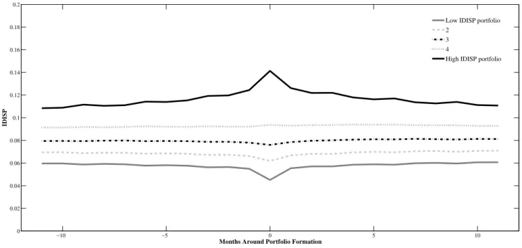
If dispersion in beliefs is a persistent rather than a random stock characteristic, the trading strategy that is necessary for exploiting the generated overpricing will require low rebalancing and hence relatively low transaction costs. To this end, we examine the average month-to-month transition probabilities for a stock, i.e. the average probability that a stock in decile portfolio i in one month will be in decile portfolio j in the next month, for ten portfolios sorted on IDISP. In Table 3, we observe that all the diagonal elements of the transition probability matrix exceed 10%, with stocks in high (low) IDISP portfolio having a huge almost 56% (40%) likelihood of remaining in the same portfolio next month. Additionally, we group stocks into quintile portfolios based on their IDISP values (from low IDISP, quintile 1 to high IDISP, quintile 5), and plot in Figure 3 the average monthly IDISP for each of the portfolios, for the eleven months before and after portfolio formation. The highest (lowest) IDISP value of 0.142 (0.045) is observed at the time of portfolio construction. Moreover, the results show a clear difference across the IDISP quintile portfolios, with a strong per-sistent ranking of the IDISP portfolios across each of the eleven months around portfolio formation. The above results indicate that IDISP is a persistent stock characteristic and far from being random.
Overall, the findings presented in this section establish a strong negative relation between IDISP and future stock returns. Moreover, they provide evidence suggesting that stocks with a high IDISP characteristic in one month also tend to exhibit high IDISP in the following months.
3.2 IDISP and Other Firm Characteristics
In this section, we study the relation between IDISP and various firm characteristics to explore the distinct information content driving the IDISP measure. We begin by examining the characteristics of firms across various IDISP portfolios. For each month, we construct decile portfolios based on
9While it is possible that some constrained pessimistic investors migrate to the options market in order to take negative positions, this does not necessarily mean that the overpricing of the underlying asset will instantly vanish. For the mispricing to be eliminated there must be actual selling/shorting activity in the equity market following the trading activity in the options market. In this spirit, Ofek, Richardson and Whitelaw (2004) compare actual stock prices with the stock prices implied by the put-call parity relation in the option market and observe widespread stock overpricing that is stronger when the underlying short-sales constraints are more severe. Grundy, Lim and Verwijmeren (2012) provide similar empirical evidence for the period of the 2008 short-sales ban.
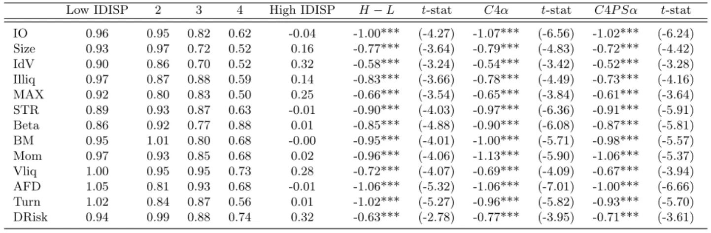
IDISP, and for each decile portfolio, we report the time-series averages of monthly mean values of all the stock-related variables examined in the study.
Table 2 (bottom panel) reports some interesting results. First, high IDISP stocks are less likely to be held by institutional investors, as suggested by the very low IO values observed for the two deciles with the highest IDISP stocks (average IO of -0.005 and -0.574 for deciles 9 and 10 respectively). The results, therefore, imply that high IDISP stocks are more difficult to short-sell (see Nagel, 2005). Second, as IDISP increases across portfolios, stocks with more dispersed beliefs tend to be relatively small, risky (both systematically and idiosyncratically, as captured by Beta and IdV, respectively), and illiquid.10 Third, high IDISP stocks show a greater propensity to exhibit lottery-type payoffs, with MAX values monotonically rising from the low IDISP to the high IDISP portfolio. The average MAX value in the lowest IDISP portfolio is 4.0%, whereas stocks in the highest IDISP portfolio have the maximum daily return over the past month of 10.9%.11 Fourth, a striking pattern is observed for book-to-market ratios – across the first nine deciles, the book-to-market ratio is similar; however it increases substantially from decile 9 (0.42) to decile 10 (0.563). This indicates a strong dominance of value stocks in the high IDISP portfolio. Fifth, comparing IDISP with the well-established proxy for beliefs dispersion among analysts’ forecasts, AFD, we document that the two measures comove uniformly across portfolios, implying cross-sectional commonalities in informational content of both dispersion measures. As IDISP increases, the average values of AFD gradually rise from 0.076 in the low IDISP portfolio to 0.50 in the high IDISP portfolio. Also, the spike from decile 9 to 10 (0.340 to 0.50) for AFD is similar to the spike observed in the IDISP measure (0.115 to 0.165). Finally, we find that firms in the highest IDISP decile portfolio exhibit higher share turnover and higher probability of default relative to the firms in the lowest IDISP portfolio, with the respective relations monotonically increasing across deciles. It is also noteworthy that the average character-istic differential between high and low IDISP portfolios is statcharacter-istically significant at the 1% level in almost all cases (the sole exception being in the case of momentum).
10
It is noteworthy that the so-called small and illiquid stocks in our optioned sample are still relatively large and liquid when compared with the full universe of stocks.
11
Since high IDISP stocks tend to have lottery-type payoffs, we also investigate whether the IDISP-return relation is affected by the January seasonality, discussed by Doran, Jiang, and Peterson (2011). Similarly to their study, we find that IDISP predicts positive returns in January. However, this relation is statistically insignificant, implying that, while IDISP shares some common features with lottery-type characteristics, its information content is distinct. This additional analysis is reported in the supplementary material online.
Next, we investigate the ability of the above firm characteristics to forecast the next-period IDISP. More specifically, we perform a Fama and MacBeth (1973) monthly cross-sectional regression of IDISP at the end of month t+ 1 on IDISP and other firm characteristics measured at the end of month t. Table 4 presents the time-series average of monthly cross-sectional coefficient estimates and correspondingt-statistics. We observe that lagged IDISP has the largest positive predictability and is highly statistically significant. This confirms the persistent nature of the IDISP measure, as observed in Table 3. More notably, we observe that IdV presents a very strong predictability for IDISP (with a t-statistic of 10.27), followed by AFD (with a t-statistic of 7.77). The fact that id-iosyncratic volatility is a strong predictor of IDISP does not come as a surprise, since it is expected that more extreme price movements will be associated with higher uncertainty about the firm’s fundamentals. In fact, Berkman, Dimitrov, Jain, Koch and Tice (2009) use IdV as another proxy for differences of opinion. The strong predictive power of AFD is also expected, since it captures the dispersion in analysts’ expectations about future earnings. With the exception of BM and Turn, all the firm characteristics examined exhibit some significant predictability for IDISP. As a result, theR2 is equal to 59%, indicating overall strong explanatory power of the characteristic variables for next-period IDISP.
In summary, the findings of this section suggest that high IDISP stocks, as compared to low IDISP stocks, are relatively small, riskier, relatively illiquid, value- (rather than growth-) oriented, with less institutional ownership, preferred by investors with lottery-type preferences, have higher analysts’ forecast dispersion and probability of default. Moreover, idiosyncratic volatility and secondarily the dispersion in analysts’ forecasts are the strongest predictors of IDISP.
3.3 Controlling for Other Cross-Sectional Characteristics 3.3.1 Bivariate Portfolio-Level Analysis
In this section, we analyze the interaction of the negative IDISP-return relationship with various stock- and option-related characteristics by performing dependent bivariate portfolio-level analysis.
Each month, we sort stocks into quintile portfolios based on one of the alternative stock- or option-related characteristics, and next, within each characteristic portfolio, we further sort stocks into five portfolios on the basis of IDISP. Finally, we compute the time-series averages of equal-weighted monthly excess returns for each of the IDISP quintiles across the five characteristic portfolios ob-tained from the first sort. This procedure of accounting for non-IDISP effects does not involve any regression-based tests and helps track the persistence of the negative IDISP effect across all char-acteristic quintiles. Additionally, we estimate the average raw returns, and the four- and five-factor alphas for the strategy that buys a high IDISP portfolio and sells a low IDISP portfolio.
The top panel of Table 5 reports the results when we control for all the stock characteristic variables considered in Tables 2 and 4. It can be seen that the IDISP effect remains strongly significant and economically substantial in all cases. This includes traditional cross-sectional return predictors such as Size, Illiq, BM or Mom but also all the newly-established characteristics that have been shown to provide negative predictability similar to that of IDISP, for example, IdV, MAX, AFD, or DRisk. The bottom panel of Table 5 presents the results when controlling for the alternative option-related predictors. We observe that the IDISP effect is robust to controlling for stocks’ risk-neutral higher moments (RNS and RNK), measures of volatility and downside risk (VolSpr and QSkew), as well as proxies of informed trading in the options market (VS, O/S, InnCall and Innput).12 Moreover, we find that the predictability of IDISP is not subsumed by that of the volatility of volatility and is also not mechanically driven by fluctuations in the level of the options trading volume.
To summarize, the findings indicate that the negative relationship between the IDISP measure and future stock returns cannot be subsumed by any of the known stock- and option-related cross-sectional return predictors documented in the literature.
12
In the supplementary material we provide further empirical evidence with respect to the relation of IDISP and informed options trading. In particular, one might hypothesize that high IDISP stocks are stocks for which there is a high options trading activity stemming from pessimistic informed investors. If this was the case, we would expect to find that the high IDISP portfolio is dominated by pessimistic trading volume. However, our results show that the trading volume in the high IDISP portfolio actually leans towards optimistic rather than pessimistic trades. Therefore, an informed trading interpretation of the predictability of IDISP is not supported by the data.
3.3.2 Fama-MacBeth Regressions
The results of the portfolio-level analyses demonstrate that a stock portfolio with high IDISP, as compared to low IDISP, generates economically substantial and statistically significant negative returns that are not subsumed by a large set of control variables. Subsequently in this section, we perform Fama and MacBeth (1973) regressions that utilize the entire cross-sectional information in the data, so as to gauge whether the IDISP-return relationship persists after simultaneously control-ling for other return predictors. In particular, each month, we perform cross-sectional regressions of excess stock returns in month t+1 on the IDISP measure and the series of previously documented return drivers, all computed in montht. We report the time-series averages of the slope coefficients, along with Newey-West correctedt-statistics (with six lags), and the R2s from the regressions. To mitigate the potential effects of outliers, we winsorize the control variables at the1st and99th per-centile.
Table 6 presents the results for all the stock- and option-related characteristics considered in the previous section. In Panel A, we estimate univariate and multivariate regression specifications of excess returns on IDISP and various stock characteristic variables. First, the univariate Fama and MacBeth model shows that the coefficient on IDISP is negative (-0.1360) and statistically significant (with a t-statistic of -3.24). The economic magnitude of the IDISP effect is similar to that pre-sented in univariate portfolio-level analysis. In particular, multiplying the difference in mean values between high IDISP and low IDISP deciles (from Table 2) by the slope coefficient yields a monthly risk premium differential between the high and low IDISP portfolio of -1.71%. Second, estimating bivariate regressions with IDISP and stock-related characteristics, the average slope coefficient on IDISP remains negative, statistically significant at the 1% level and economically large, with values ranging between -0.1338 and -0.1040. Of all stock-related characteristics, the residual institutional ownership, the idiosyncratic volatility and the distress risk exhibit a statistically significant pre-dictability for future stock returns after controlling for IDISP, with the signs of their coefficients being consistent with Nagel (2005), Ang, Hodrick, Xing and Zhang (2006) and Gao, Parsons and Shen (2018), respectively. Interestingly, AFD does not exhibit any significant cross-sectional pre-dictability after controlling for IDISP, even though it is significant (at the 5% level) in the univariate
model. Finally, in the multivariate model specification with all the control variables, we observe that IDISP retains its significance (t-statistic of -2.31), with a slope coefficient value of -0.0543. In economic terms, this coefficient translates to a return differential of -0.68%.
In Panel B, we provide the predictability results from univariate and multivariate regression speci-fications involving IDISP and other option-related characteristic variables which were considered in the previous section. We observe that in bivariate regressions, the coefficient on IDISP is statisti-cally significant at the 1% level in all but one case (when controlling for VoV, where it is significant at the 5% level), and economically substantial, with values ranging between -0.1366 and -0.1025. From the remainder of the variables, RNS and VS exhibit a positive and significant effect, consistent with the findings of Stilger, Kostakis and Poon (2017) and Cremers and Weinbaum (2010) respec-tively, while QSkew, O/S, InnPut and VoV exhibit a negative and significant effect, in line with the studies of Xing, Zhang and Zhao (2010), Johnson and So (2012), An, Ang, Bali and Cakici (2014) and Baltussen, Van Bekkum and Van Der Grient (2015), respectively. When all option-based char-acteristics are jointly considered in the regression specification, we observe that the slope coefficient associated with IDISP remains negative (-0.0697) and retains its statistical significance (t-statistic of -2.10). In economic terms, this coefficient translates to a return differential of -0.88%.
Overall, the Fama and MacBeth regression results confirm that the IDISP measure has strong explanatory power for future excess stock returns, which is robust to that of a wide range of stock-and option-related characteristics.
4
Dissecting the Predictability of IDISP
In this section, we delve into understanding the economic nature of the negative predictability of the IDISP measure. In particular, we investigate how the IDISP effect relates to short-selling impediments, earnings announcements and periods of market-wide optimism.
4.1 IDISP Effect and Short-Selling Impediments
Miller’s (1977) theory predicts that stocks with a high dispersion of opinions tend to be overpriced and are expected to earn negative subsequent returns. However, a necessary condition for this overpricing to be generated is that there are high costs associated with short-selling that prevent pessimistic investors from taking negative positions. In addition, the reason the overpricing persists and is not instantly eliminated is due to the inability (or reluctance) of the average investor to short-sell the stock. Therefore, if the negative predictability of IDISP is indeed related to diver-gence of opinions leading to an overpricing, we would expect to find that the effect is stronger when short-selling is more costly and more difficult in the presence of limits to arbitrage.
To test this economic prediction, we use the level of residual institutional ownership (IO), market capitalization (Size), idiosyncratic volatility (IdV) and illiquidity (Illiq) as the dimensions commonly associated with shorting constraints and limits to arbitrage. Intuitively, the lower the level of insti-tutional ownership, the lower the supply for loanable shares by institutions (Nagel, 2005) and hence the higher the fee that the short-seller needs to pay. Similarly, relatively small, volatile and illiquid stocks exhibit more severe limits to arbitrage (Shleifer and Vishny, 1997; Pontiff, 2006; Sadka and Scherbina, 2007; Gromb and Vayanos, 2010; Conrad, Kapadia and Xing, 2014) and hence investors are less willing to short-sell such stocks and exploit the mispricing.13
For the empirical investigation, we perform a dependent bivariate portfolio-level analysis. More specifically, each month we first sort stocks in ascending order into tercile portfolios on the basis of key firm characteristic variables associated with short-selling impediments, and next, within each characteristic portfolio, we further sort stocks into quintile portfolios based on IDISP values. Fi-nally, for the resulting fifteen characteristic-IDISP portfolios, we calculate equal-weighted average future monthly excess returns and present a time-series average of these values over all the months in our sample. We also evaluate the average returns, four-factor and five-factor (after augmenting Carhart’s model with the liquidity factor) alphas for the strategy that buys high IDISP stocks and
13Given that shorting constraints and limits to arbitrage are unobservable quantities, we base our analysis on various proxies that the prior literature has suggested. While it is plausible that our proxies are to some extent related to information asymmetry, we show earlier that the predictability of IDISP is unlikely to be driven by informed trading (see Section 3.3 and the discussion in the supplementary material).
sells low IDISP stocks within each characteristic portfolio quintile.
Table 7 reports the results. We observe that the high IDISP portfolio underperforms the low IDISP portfolio by 1.77% per month (with a t-statistic of -3.06) if these firms have a low level of IO, whereas the return differential is only -0.61% per month (with an insignificant t-statistic of -1.41) for high IO firms. Moreover, the return differential decreases monotonically (in absolute terms) as we move from the low IO tercile to the high IO tercile. In line with the theoretical predictions of Miller (1977), the negative performance is mainly driven by high IDISP firms that appear in the lowest IO terciles. In particular, the high IDISP firms in the lowest IO portfolio earn on average -0.83% per month in excess of the risk-free rate, while high IDISP stocks with higher levels of IO earn instead a return premium. The idea that the IDISP effect is more pronounced among stocks with high short-sale costs is also confirmed when controlling for asset-pricing risk factors. More specifically, we observe that both the four- and five-factor model alpha spreads between high IDISP and low IDISP portfolios become larger (in absolute terms) and more statistically significant as we move from high to low IO firms. For example, the monthly five-factor alpha of the H−L IDISP portfolio is -1.83% (with a t-statistic of -4.82) if the stocks in this portfolio are more difficult to short-sell, while high IDISP stocks underperform low IDISP stocks by 0.54% (with at-statistic of -1.85) if one can short-sell these stocks at a relatively low cost. It is also important to note that the difference in theH−LIDISP portfolio alphas between high IO and low IO firms is statistically significant at the 1% level (t-statistic of 2.95).
Further, we observe that the underperformance of high IDISP relative to low IDISP stocks is most pronounced when considering low market capitalization (-1.42% per month with a t-statistic of -3.33), high idiosyncratic risk (-1.86% per month with at-statistic of -4.34) and low liquidity stocks (-1.42% per month with at-statistic of -3.24). On the other hand, the returns on theH−Lportfolio are negligible and statistically insignificant for big, less risky and more liquid firms. In fact, the negative return differentials decrease in absolute terms (or even turn positive) almost monotoni-cally as we move further away from the portfolios with the smallest, most volatile and least liquid stocks. In addition, we find that the negativeH−LIDISP portfolio returns mainly stem from high IDISP firms that appear in the lowest tercile of market capitalization and the highest terciles of
idiosyncratic volatility and illiquidity. More specifically, high IDISP stocks in the lowest capitaliza-tion, highest idiosyncratic volatility and highest illiquidity portfolios earn average monthly excess returns of -0.40%, -1.11% and -0.48%, respectively. On the other hand, high IDISP stocks with high size, low volatility and high liquidity earn instead a large return premium. The result indicates that the underperformance of high IDISP stocks is pronounced for stocks that exhibit high arbitrage risk.
After controlling for asset-pricing risk factors, the four-factor and five-factor alphas remain eco-nomically substantial and highly significant for the portfolios with the smallest, most volatile and most illiquid stocks, while they become negligible and insignificant as we move further away from those portfolios. For example, the five-factor alpha differential between high IDISP and low IDISP portfolios is equal to -1.25% per month (with a t-statistic of -2.94) for low Size, -1.69% per month (with a t-statistic of -4.14) for high IdV and -1.25% per month (with a t-statistic of -3.22) for high Illiq stocks. By contrast, the risk-adjusted (by the four- or five-factor model) returns on the
H−L IDISP portfolio remain small and statistically insignificant for high Size, low IdV and low Illiq portfolios. Moreover, the difference in theH−LIDISP portfolio alphas between high arbitrage risk firms and low arbitrage risk firms is statistically significant in all cases.
Overall, our results provide strong supportive evidence in favor of the role that shorting constraints and limits to arbitrage play in explaining the substantial return variations in high and low IDISP portfolios. Therefore, they are in line with the notion that the predictability of IDISP is associated with overpricing caused by increased dispersion in investors’ opinions.
4.2 IDISP Effect around Earnings Announcements
Our empirical findings display systematically low returns for high IDISP stocks, which is expected when IDISP serves as a proxy for differences in expectations among investors. Quarterly earnings announcements feature fertile grounds for validating IDISP’s information content. In particular, they constitute a firm-specific corporate event whereby optimistic and pessimistic investors specu-late on the forthcoming earnings outcome (see, for example, Kim and Verrecchia, 1991; and Kandel and Pearson, 1995). In this regard, earnings announcements ideally fit within the stylized
frame-work presented in Appendix A. Moreover, in the presence of short-sales constraints, the net effect of intensified speculative trading on prices is expected to be positive and should cause stocks to be-come overvalued in days preceding the earnings announcements, with higher differences of opinion leading to overvaluation. However, in the post-announcement period, the release of new informa-tion about earnings reduces differences in expectainforma-tions among investors, and consequently, these announcements contribute to the reduction in overvaluation (Berkman, Dimitrov, Jain, Koch and Tice, 2009). As such, we would expect a particularly pronounced negative IDISP-return relationship surrounding the quarterly earnings announcements.
We investigate the above proposition using earnings announcement dates obtained from the Com-pustat Quarterly file for all available optionable stocks in our sample. For this analysis IDISP is estimated by averaging daily IDISP values within a month ending 10 trading days prior to the earn-ings announcement date (IDISP(−31,−10)). In this fashion, IDISP is constructed from trading dates
data available prior to earnings announcements and discards information up to two weeks prior to the announcement date to preclude possible contamination of the measure from investors who might trade options in order to capitalize on excessive volatility usually observed around such announce-ments (see, for example, Frazzini and Lamont, 2007). For robustness, we also estimate another two ex-ante IDISP versions, one that spans a month ending 2 trading days prior to the announcement (IDISP(−23,−2)) and one ending 5 trading days prior to the announcement (IDISP(−26,−5)).
To empirically investigate whether high IDISP stocks earn significantly lower returns around earn-ings announcements than low IDISP stocks, we follow in spirit the setting of Berkman, Dimitrov, Jain, Koch and Tice (2009). In particular, we estimate the average excess earnings announcement period returns for quintile portfolios formed using each of the three IDISP measures and also report the average excess returns for the portfolioH−Lthat buys high IDISP stocks and sells low IDISP stocks. Excess returns are estimated as the difference between the buy-hold stock returns and the value-weighted CRSP index buy-hold returns, over the three trading days surrounding the earnings announcement date.14 Table 8 displays the findings, showing that high IDISP stocks underperform low IDISP stocks by an economically large and statistically significant average announcement excess
14
return ranging from 0.73 to 0.80%.15
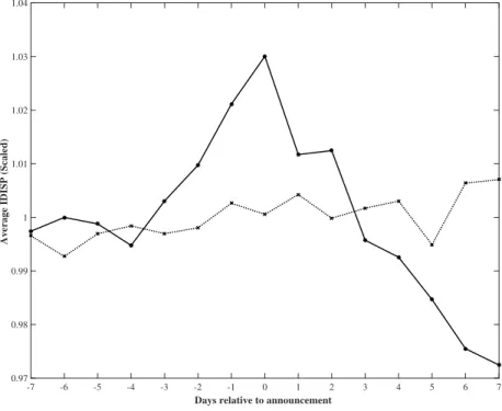
Next, we study the dynamics of the IDISP measure around the earnings announcement dates by plotting the average daily IDISP values across all firms and announcements in our sample for the period covering seven days before and after the event date.16 Figure 4 shows that the average IDISP exhibits an upward trending pattern in the period before the event, reaching its maximum value on the earnings announcement day. Following the announcement, it exhibits a dramatic decline as the uncertainty pertained to earnings is resolved. To further scrutinize the interaction between IDISP and earnings announcements, we also plot the average daily IDISP values across firms around a pseudo-event date that is selected randomly from the one-month period starting one month after the actual announcement date. As expected, Figure 4 shows that IDISP does not exhibit any sys-tematic pattern around the pseudo-event date.
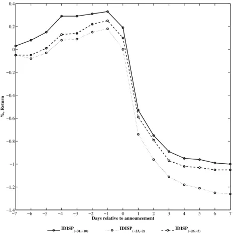
Finally, we plot the average cumulative excess returns for the H−L portfolio over the same 15-trading-day period surrounding the earnings announcements. This analysis allows us to visualize the asymmetric effects of differences in expectations which should stimulate a price run-up for high IDISP stocks resulting in overpricing in the pre-announcement period, subsequently followed by a price correction in the post-announcement period. Figure 5 illustrates the results showing that the
H−L IDISP portfolio exhibits a large price run-up, as high as 0.33% over the 7-day period prior to the announcement, followed by a substantial price reversal, reaching as low as -1% by the end of the event window.
Summing up, we observe that the IDISP effect is particularly pronounced around earnings an-nouncements. Moreover, the average daily IDISP measure exhibits an increasing pattern before an announcement and experiences a dramatic drop right after the event. We interpret these findings as evidence to support that IDISP indeed captures dispersion in beliefs among investors.
15
In the supplementary material we show that the observed IDISP return predictability around earnings announce-ments is also not subsumed by various proxies of informed trading.
16We use only those firms’ announcements for which IDISP values exist for all the 15 days under examination. Moreover, for better comparability, the daily IDISP values of each firm are scaled by the respective firm’s average IDISP across the examination period.
4.3 IDISP Effect and Investor Sentiment
The negative relation between dispersion in beliefs and stock returns can be explained in the context of a market where short-sale constraints make it difficult for pessimistic investors to take negative positions and hence prices reflect only the views of the optimistic investors who end up holding the stock. As Stambaugh, Yu and Yuan (2012) postulate, when market-wide sentiment is high, the views of those investors who finally hold the asset tend to be excessively optimistic, resulting in a severe overpricing. On the other hand, when market-wide sentiment is low, the views of those investors who finally hold the asset are closer to being rational, and hence a pronounced overpricing is less probable. This implies that the negative relation between disagreement and stock returns is expected to stem mainly from periods of high sentiment in the market.17,18 In this regard, we test whether the predictability of IDISP is consistent with the above premise by investigating the IDISP effect separately for times of high and low investor sentiment. In particular, we estimate monthly cross-sectional Fama and MacBeth (1973) regressions separately for high and low sentiment periods. Following Stambaugh, Yu and Yuan (2012), we define high (low) sentiment months as those when the Baker and Wurgler (2006) index in the previous month is above (below) the median value in the sample.
Table 9 presents the Fama and MacBeth (1973) slope coefficients for IDISP from the various re-gression specifications after controlling for stock- and option-related characteristics in high and low sentiment periods. In the panel with stock characteristics results, Model (1) shows univariate regres-sion with IDISP, Models (2)-(14) show bivariate regresregres-sions with IDISP and the stock characteristic variable listed in the column header and Model (15) is the multivariate regression with IDISP and all the stock characteristic variables. Similarly, in the panel with option characteristics results, Models (1)-(10) show bivariate regressions with IDISP and an option characteristic variable, and Model (11) is the multivariate regression with IDISP and all the option variables. The results provide a consistent picture across all the regression specifications. Following periods of high sentiment, we
17Atmaz and Basak (2018) create a theoretical model which predicts that even without short-sale constraints, the negative relation between dispersion in beliefs and future returns should stem from optimistic periods.
18Recent studies that emphasize the importance of conditioning on market-wide investor sentiment for explaining asset prices include Yu and Yuan (2011), Stambaugh, Yu and Yuan (2012) and Antoniou, Doukas and Subrahmanyam (2015).
observe that the slope coefficients for IDISP are economically large, with strong statistical signifi-cance. The univariate analysis produces a significant (at the 1% level) slope coefficient of -0.2147 for the high sentiment period, compared to -0.0573 (and insignificant) for the low sentiment period. After controlling for various stock and option characteristics, IDISP retains its strong negative pre-dictability for excess returns in high sentiment months. The effect is negligible following times of low sentiment, where the negative IDISP-return relationship remains statistically insignificant in most specifications. Furthermore, in the majority of the specifications (20 out of 26) the difference in the IDISP coefficients between high and low sentiment periods is statistically significant as well.
Overall, the findings confirm that the IDISP effect mainly stems from periods of high investor sentiment. This is in accordance with the notion that IDISP reflects investors’ dispersion in beliefs which, in the presence of binding short-sales constraints, leads to overpricing.
5
Additional Analysis
This section complements the main findings in the paper by, first, examining the robustness of the IDISP-return predictability using signed volume data and various alternative empirical measurement definitions, and second, testing the IDISP-return relation for longer predictability horizons.
5.1 Construction of the IDISP Measure with Signed Volume Information
As discussed in Section 2.1 and Appendix A, the interpretation of IDISP as a proxy for dispersion in beliefs relies on the notion that, in the typical stock options trading environment, investors’ optimal moneyness levels are proportional to their optimistic or pessimistic beliefs. In particular, investors with more optimistic (pessimistic) views will elect to either buy more OTM calls (puts) or sell more ITM puts (calls). While this theoretical prediction also holds for cases where the above strategies are replicated synthetically by purchasing matched-strike ITM puts (calls) and selling matched-strike OTM calls (puts) respectively, it is unclear how many investors actually implement such complicated put-call parity strategies. Moreover, Appendix A shows that in some cases it might be optimal for option buyers with slightly optimistic or pessimistic expectations to trade ITM rather than OTM options. Therefore, it is important to check the validity of our previously
presented results using an alternative IDISP measure that utilizes signed volume data and more specifically only the buy-side trading volume of OTM options and the sell-side trading volume of ITM options. In other words, we use only the trading volume across different moneyness levels that reflects expectations more clearly, i.e. we retain only OTM call purchases and ITM put sales, which are undoubtedly optimistic trades related to positive expectations, and OTM put purchases and ITM call sales, which are undoubtedly pessimistic trades related to negative expectations.
To this end, we collect signed options volume data from the International Securities Exchange (ISE) Trade Profile. This dataset contains all end-users’ trades disaggregated by whether each trade is a buy or a sell order. In the majority of cases, a market maker provides liquidity by being on the other side of the trade. While the ISE options volume data represent about 30% of the total individual stock options trading volume across all options exchanges, Ge, Lin and Pearson (2016) show that the data are representative of the total options volume provided by OptionMetrics. Since the ISE data are only available for a much shorter period (from May 2005 onwards), we consider the results obtained in this section as complementary to, and supportive of, those presented in the main em-pirical analysis. Hence, the IDISP measure constructed from signed volume can be seen as a robust version of the original measure presented in the paper. It is also important to note that, unlike signed volume data, daily unsigned volume data are publicly available and hence easily accessible to investors. Therefore, the usage of unsigned volume data in the main empirical analysis highlights the fact that a trading strategy based on the predictive power of IDISP would be relatively cheap and implementable by an investor in real time.
Table 10 displays equal- and value-weighted return predictability results for the new IDISP portfo-lios constructed with the ISE signed options volume. The results display a consistent picture, with returns that are of similar economic magnitude and statistical significance to those presented in Ta-ble 2. Moreover, we observe a striking resemblance in the return properties of the decile portfolios sorted on the new IDISP measure, with the largest decline in the average monthly excess return observed from decile 9 to decile 10. Further, the H−L portfolio return is -1.28% per month for equal-weighted portfolios and -1.21% per month for value-weighted portfolios, significant at the 5% and 10% levels respectively. In line with Table 2, the results become stronger when considering
risk-adjusted returns. For example, the five-factor alpha differential between high and low IDISP stocks is -1.66% and 1.67% per month for equal- and value-weighted portfolios, with t-statistics of -5.74 and -4.99 respectively. Overall, the findings suggest that the IDISP measure, capturing the trading activity at various moneyness levels, exhibits consistent negative predictability for the cross-section of stock returns, irrespective of whether we use unsigned or signed trading volume data.
5.2 Alternative Constructions of the IDISP Measure
Next, we test whether the negative IDISP-return relationship is robust to alternative definitions of dispersion. Hence we construct IDISP measures based on mean absolute deviations and standard deviations, of moneyness levels as well as strike prices. Additionally, we consider IDISP specifica-tions using alternative screening criteria on the minimum number of days with non-missing IDISP values and inclusion of near-the-money options in the IDISP computation. Finally, we obtain results for IDISP measures estimated without averaging within a month.
Thus, we construct nine alternative IDISP measures. IDISP1 is the standard deviation of stock options trading volume across moneyness levels. IDISP2 and IDISP3 are mean absolute and stan-dard deviation measures respectively, of options trading volume across strike prices (rather than moneynesses), scaled by the volume-weighted average strike. IDISP4 and IDISP5 are similar to the original IDISP measure and to IDISP1 respectively, but we use alternative filtering criteria requir-ing within a month at least ten days of non-missrequir-ing IDISP values. IDISP6 and IDISP7 are similar to the original IDISP measure and to IDISP1 respectively, but we include near-the-money options in calculating the measures. IDISP8 and IDISP9 are similar to the original IDISP measure and to IDISP1 respectively, but are measured at the penultimate day of a month (instead of averaged within a month excluding the last trading day).
Table 11 reports the average equal-weighted returns of portfolios with the lowest and highest IDISP in the previous month. For all nine alternative IDISP measures, we observe that the portfolios with the highest IDISP values consistently underperform the lowest IDISP portfolios, both on a raw return as well as a risk-adjusted return basis. For instance, the five-factor alpha differential between