Center for Policy Research Maxwell School of Citizenship and Public Affairs
Fall 12-2015
The Behavioral Impacts of Property Tax Relief: Salience or
The Behavioral Impacts of Property Tax Relief: Salience or
Framing?
Framing?
Phuong Nguyen-Hoang
University of lowa, [email protected] John Yinger
Syracuse University, [email protected]
Follow this and additional works at: https://surface.syr.edu/cpr
Part of the Behavioral Economics Commons, Income Distribution Commons, and the Public Affairs, Public Policy and Public Administration Commons
Recommended Citation Recommended Citation
Nguyen-Hoang, Phuong and Yinger, John, "The Behavioral Impacts of Property Tax Relief: Salience or Framing?" (2015). Center for Policy Research. 221.
https://surface.syr.edu/cpr/221
This Working Paper is brought to you for free and open access by the Maxwell School of Citizenship and Public Affairs at SURFACE. It has been accepted for inclusion in Center for Policy Research by an authorized administrator of SURFACE. For more information, please contact [email protected].
The Behavioral Impacts of
Property Tax Relief: Salience or
Framing?
Phuong Nguyen-Hoang and John Yinger
Paper No. 186__________
Associate Professor of Public Administration and International Affairs (PAIA)
Associate Directors
Margaret Austin Associate Director Budget and Administration
John Yinger
Trustee Professor of Economics and PAIA Associate Director, Metropolitan Studies Program
SENIOR RESEARCH ASSOCIATES Badi H. Baltagi... Economics
Robert Bifulco ... PAIA Leonard Burman ... PAIA Thomas Dennison ... PAIA Alfonso Flores-Lagunes ... Economics Sarah Hamersma ...PAIA William C. Horrace ... Economics Yilin Hou ... PAIA Hugo Jales... Economics Duke Kao... Economics Jeffrey Kubik... Economics Yoonseok Lee ... Economics Amy Lutz... Sociology
Yingyi Ma ...Sociology Jerry Miner ...Economics Cynthia Morrow ... PAIA Jan Ondrich...Economics John Palmer... PAIA David Popp ... PAIA Stuart Rosenthal ...Economics Rebecca Schewe ...Sociology Amy Ellen Schwartz ... PAIA/Economics Perry Singleton………...Economics Michael Wasylenko ... ……….Economics Peter Wilcoxen...…PAIA
GRADUATE ASSOCIATES Emily Cardon ... PAIA
Brianna Carrier ... PAIA John T. Creedon... PAIA Carlos Diaz ...Economics Alex Falevich ...Economics Wancong Fu ...Economics Boqian Jiang ...Economics Yusun Kim ... PAIA Ling Li ...Economics Michelle Lofton ... PAIA Judson Murchie ... PAIA Brian Ohl... PAIA Jindong Pang ...Economics Malcolm Philogene ... PAIA William Reed ... PAIA
Laura Rodriquez-Ortiz ... PAIA Fabio Rueda De Vivero ... Economics Max Ruppersburg ...PAIA Iuliia Shybalkina ...PAIA Kelly Stevens ...PAIA Mary Stottele... PAIA Anna Swanson...PAIA Tian Tang...PAIA Saied Toossi ...PAIA Rebecca Wang ... Sociology Nicole Watson... Social Science Katie Wood ...PAIA Jinqi Ye ... Economics Pengju Zhang ...PAIA Xirui Zhang ... Economics STAFF
Kelly Bogart...….………...….Administrative Specialist Mary Santy..….…….….……....Administrative Assistant Karen Cimilluca...….….………..…..Office Coordinator Katrina Wingle...….……..….Administrative Assistant Kathleen Nasto...Administrative Assistant
from school property taxes. From 2006-07 to 2008-09, these exemptions were supplemented with rebates, which arrived as a check in the mail. The purpose of this paper is to determine whether these two algebraically equivalent but administratively distinct policies of tax relief led to different behavioral responses. Drawing on behavioral economics, we explore the impact of STAR on the price elasticity of demand for school quality based on the concepts of salience and framing. Our main results are that the behavioral impact of the STAR provisions are larger (1) when they are most salient and (2) when they are framed as a property tax reduction instead of as unlabeled income. We also show that salience and framing can help to explain flypaper effects linked to state educational aid and to the resources that are freed up by a decline in the price of education.
JEL Codes: H31, H71, H75
Key Words: Property Tax Relief, Demand for Education, Salience, Framing, Flypaper Effects
The authors are, respectively, Assistant Professor of Urban and Regional Planning, University of Iowa; and Professor of Economics and Public Administration, The Maxwell School, Syracuse University. We are grateful for helpful suggestions from Tatiana Homonoff as we were starting this project and to Eric Brunner and Joshua Hymen for helpful comments on earlier drafts. Phuong Nguyen-Hoang, School of Urban and Regional Planning, University of Iowa, Iowa City, IA 52242, 319-335-0034, [email protected]
John Yinger (Corresponding Author), Center for Policy Research, 426 Eggers Hall, Syracuse University, Syracuse, NY 13244, 315-443-9062, [email protected].
exemptions for homeowners in a form equivalent to a matching grant. From FY2006-07 to FY2008-09, these exemptions were supplemented with mailed rebate checks that took the same form. The STAR exemptions and rebates alter voters’ tax shares for education. Our main objective is to determine whether the associated price elasticity of demand for education is different for these two algebraically equivalent but administratively distinct forms of tax relief, and, if so, whether the difference can be explained by the concepts of salience and framing.
These two concepts are drawn from the literature on behavioral public finance, much of which has been inspired by Chetty, Looney, and Kroft (2009; CLK for short). CLK ask whether the behavioral impact of tax provisions depends on the “salience” of those provisions, where salience is defined as visibility or prominence.1 As discussed below, CLK and several other
studies find an affirmative answer to this question, and we provide a new way to address it. Our analysis also complements the Cabral and Hoxby (2012) study of property tax salience based on the use of escrow accounts, and other studies on whether behavioral responses to new resources depend on the household mental account in which those resources appear—a type of framing.
Although our focus is on the natural experiment created by the temporary STAR rebate program, similar issues arise with other components of the local tax price for education. Price elasticities for different components of tax price were estimated by Eom et al. (2014). This paper builds on the Eom at al. framework and explores whether salience and framing can help to explain differences in price elasticities across tax-price components. This approach also makes it possible to look for signs of salience and framing in flypaper effects, which arise when lump-sum education aid has a larger impact on education demand than an equivalent (defined below)
amount of voter income. Thus, we contribute to the literature on state aid by estimating different flypaper effects under different circumstance. In addition, we introduce a new type of flypaper effect that appears in the income effect associated with a STAR-induced price change, and we compare this flypaper effect with the one linked to state aid.
We begin with a description of the STAR program. Then we turn to the concepts of salience and framing. We review the literature on the impact of these concepts on behavioral responses to taxes, and we explain how they apply to the behavioral responses to provisions in STAR. We explain how salience and framing may affect the price elasticity of education demand and show that flypaper effects may appear in this price elasticity through the income effect. We also show that the concepts of salience and framing can help to explain both responses to non-STAR components of tax price and traditional (state aid) flypaper effects. The next section explains our estimating procedure, data, measures, and robustness checks. We then present the results of our hypothesis tests concerning salience and framing, including hypotheses about both the STAR and the non-STAR components of tax shares and traditional flypaper effects. Finally, we summarize our main results and discuss their key policy implications.
STAR History and Design of STAR
The STAR program provides homestead exemptions from school-district property taxes for owner-occupied primary residences.2 NYS funds these exemptions by compensating school districts for the lost revenue. According to DiNapoli (2013, 6), STAR “provided almost 3.4 million exemptions in 2010-11,” and STAR is expected to cost NYS “over $3.7 billion by 2015-16.” STAR does not provide property tax relief to renters or commercial and industrial property.
the basic exemption, which applies to any primary residence, including one-, two-, and three-family houses, condominiums, cooperative apartments, mobile homes, and residential dwellings in mixed-use property. Before adjustments (described below), the basic exemption is $30,000, although it was phased during 1999-00 ($10,000) and 2000-01 ($20,000). A homeowner’s assessed value is reduced by the exemption, so the amount it saves equals the exemption multiplied by the school property tax rate in the school district where the house is located.
STAR has special provisions for homeowners in the “big-five” school districts, New York City (NYC), Buffalo, Rochester, Syracuse, and Yonkers, because these districts are not independent but instead are city government departments. The STAR exemption is half of the basic exemption in NYC and two-thirds of the basic exemption in the other four districts. Because these districts do not have separate school taxes, their exemptions apply to all city property taxes. Unlike other districts, NYC raises much school revenue from an income tax, so the STAR legislation also created an income tax credit for all NYC residents, including renters.
Homeowners aged 65 or above with income below a certain limit are eligible for the enhanced exemption. Both the exemption amount and the income limit have varied over time. In 2013-2014, the exemption amount was $63,300 and the income limit was $83,300. An income limit of $500,000 was also added to the basic STAR in 2011-12. Starting in 2011-12, an individual’s STAR tax savings could not increase by more than 2 percent per year.3
The STAR exemptions are adjusted to account for variation in assessing practices across districts. This adjustment allows us to model the STAR exemptions as an amount subtracted from a property’s market value. In addition, STAR exemptions are multiplied by a “sales price differential factor” (SPDF), which is the greater of 1.0 and the median residential sale price in a district’s county relative to the statewide average sales price. The SPDF increases STAR
exemption in counties with relatively high property value. These counties are mostly located in “downstate” NYS, which includes NYC and its suburbs plus the rest of Long Island.4
In its 2006-07 budget, NYS introduced the Local Property Tax Rebate Program, LPTRP: Local property taxpayers who receive either the basic or enhanced STAR exemption and paid their school taxes will receive rebate checks equal to $9,000 multiplied by the product of the school district tax rate and the county sales price differential factor, if any. Senior citizens that qualify for the enhanced STAR exemption receive a rebate as
computed above times 1.67. There is also an adjustment factor for qualified taxpayers whose residences are in the Big 5 city school districts (NYS Department of Taxation and Finance, NYSDTF, 2006)
In other words, LPTRP was algebraically equivalent to a 30 percent ($9,000/$30,000) increase in the basic STAR exemption. In 2007-08 and 2008-09, the LPTPR was modified to be a higher percentage of STAR savings for lower-income households and to have an income ceiling of $250,000. The LPTPR was repealed in 2009.
The STAR exemptions appear on a homeowner’s school property tax bill, whereas LPTRP took the form of a rebate check sent by mail. According to NYSDTF (2006):
The Office of Real Property Services (ORPS) is responsible for assembling the list of eligible real property owners from the final assessment rolls provided by local assessors by July 31st. ORPS then provides the list of rebate-eligible parcel owners, the mailing addresses and information necessary for the computation of the rebate amount to the Tax Department no later than August 15th. The Department must issue checks to the extent possible, by October 31st.
Administration of STAR
STAR was signed into law by Governor George E. Pataki in August 1997. Elderly homeowners received “enhanced” STAR exemptions in the 1998-99 school year, and “basic” exemptions for all homeowners were phased in from 1999-00 to 2001-02. Each district was required to notify all homeowners in the district about the existence of STAR and the need to apply for the STAR exemption. School officials had incentives to implement this requirement; each STAR exemption that was granted was fully funded by NYS. In many cases, cities and
towns also sent out notices, and newspapers publicized the sign-up requirements (Greene 1998).5
The application procedure was relatively simple. Homeowners had to fill out a one-page form to establish their residency and ownership. See Figure 1. This form was available from the local assessor (with whom it had to be filed) and on the NYSDTF web site. The form was also included in mailings to homeowners by school districts or other local governments, and NYSDTF posted online a pamphlet and other information about STAR. Once filed, the STAR form did not need to be re-submitted in later years. Data on participation rates over time are not available, but these rates can be approximated by comparing the number of STAR exemptions with the number of owner-occupied housing units in the state. By this measure, the participation rate was 68.1 percent in 2000 and rose to 86.8 percent in 2010.6
In most districts, STAR applications are due by March 1 and tentative assessment rolls (or TARs) for the following school year are announced by May 1. These TARs must be posted on the community assessor’s web site. Homeowners must be notified about an increase in their assessment, but otherwise it is homeowners’ responsibility to look up their tax liability. The TAR also provides information on a homeowner’s STAR exemption based on the latest SPDF. See the first panel of Figure 2.7 The SPDFs are certified sometime between the tax bill in September and the announcement of the TAR in the following May 1 (NYSDTF 2015c).
Homeowners usually have until the fourth Tuesday of May to appeal their assessment to their assessor. If the assessor denies the appeal, they can bring a claim in small claims court or file a lawsuit (NYSDTF 2015a). The final assessment roll is usually announced on July 1. Voter decisions are made in the school district budget votes, which are scheduled on the third Tuesday of May. Districts are required to hold a public hearing on the proposed budget during the two weeks preceding this vote and to provide voters with information about the budget proposal.8
In most districts, property tax bills are mailed in early September. The STAR legislation includes a Taxpayer Bill of Rights, which requires districts to include information about a taxpayer’s STAR exemption and the associated tax savings on the school property tax bill.9 Figure 3 provides an example, with boxes added around the STAR information. The state
provided software to prepare the first STAR tax bills, and in 2000-01 handed out $10.4 million in aid “to help localities defray the cost of processing STAR exemption applications and modifying tax bills to comply with the Taxpayer’s Bill of Rights” (McCall 2001, 23). For the first vote with the basic STAR in May 1999, non-elderly homeowners had not yet received a property tax bill with STAR information, but STAR had been extensively publicized and it did appear on the TAR that year. Basic STAR information first appeared on tax bills in September 1999 (Figure 3).
Governor Pataki proposed a STAR rebate program in his executive budget in early 2006. The legislature passed an alternative version, which Governor Pataki vetoed. As a result, no rebate program was in place for the school budget votes in late May, 2006 (Gormley 2006). After further negotiation, however, Governor Pataki and the state legislature agreed on a rebate
program, which was included in the budget signed into law on June 23, 2006. These rebates were given to every household with a STAR exemption, with no required application. Eventually, 3.4 million rebate checks were sent (MilGrim 2006). Although this program was not in existence when the 2006 school budget votes took place, some voters may have anticipated it because both Governor Pataki and the state legislature had championed the concept.
The rebate program was announced to all homeowners in the fall of 2006 in the form of rebate checks. The mailing list for these checks was provided to NYSDTF by local assessors. According to one account, these checks “arrived at voters’ homes just before the November election day. And coinciding with the checks were taxpayer-funded newsletters from lawmakers,
informing constituents that the checks were on the way” (Precious 2013). Another account revealed that each rebate check was accompanied by a note indicating that it was “approved by Gov. George Pataki and the state Legislature” (Karlin 2014).
In 2007, the new governor, Eliot L. Spitzer, proposed, and the legislature passed, a new rebate, called Middle Class STAR, that varied with income.10 Thanks to the income
conditioning, a new round of applications was required. Between July and October of 2007, over 2.7 million notices and applications were mailed to basic STAR recipients, 79 percent of whom then filed applications online or by mail (NYSDTF 2007). Reminders were also sent to 600,000 homeowners. The final participation rate was close to 90 percent (Spitzer 2008). Information about the rebate did not appear on property tax bills in any of the affected years. Moreover, the rebate was not listed on the TAR, although some jurisdictions apparently included the rebate in the listed STAR exemption. Figure 2 shows an example of a jurisdiction with the basic STAR exemption in 2006 and a much larger exemption in 2008, when the rebates were in place.11
The application procedure was simple. “To receive a rebate check, homeowners only have to verify the property information provided on the application, enter the names, social security numbers, and all required information for all resident property owners and their spouses, verify the mailing address, and submit the application” (NYSDTF 2007). Even though income information was used in determining the rebate, income did not have to be included on the application, because the taxpayer’s SSN allowed state officials to match the taxpayer with an income tax form. With this procedure, homeowners did not need to reapply for their 2008 rebate.
In addition to its coordinated mailings and press releases around the state, NYSDTF also set up a web site, which had 4 million hits that year, and three-quarters of the applications were submitted online (Spitzer 2008, 208). As a result of these efforts, about 2.3 million rebate checks
were mailed to non-senior homeowners for 2007-08 (NYSDTF 2008a). By Dec 5, 2008, 2.9 million 2008-09 rebate checks were sent to all eligible taxpayers (NYSDTF 2008b).
In summary, the STAR rebate program was not in place for the school budget votes in May 2006, although it may have been anticipated. The 2006-07 rebates went to all taxpayers with a STAR exemption, without the need for an application. Rebates were in place for the budget votes in May 2007, but taxpayers had not yet filled out the new, required application for the 2007-08 income-based rebate. They therefore knew about the rebate, but perhaps were not aware that it would be continued. Rebates were also in place for the budget votes in May 2008. By this time voters had received the rebates for two years and filled out an application. No additional application was needed to receive these rebates in the fall of 2008. The rebates were repealed before the school budget votes in May 2009 (Office of Tax Policy Analysis 2009).
Salience and Framing Concepts and Existing Evidence
The literature on behavioral economics provides two helpful concepts to explain why behavioral responses to STAR may depend on the way STAR is administered: salience and framing. First, a salient policy is one that is visible. Standard economic analyses generally assume that consumers or taxpayers have perfect information and that they pay attention to, and take into account, taxes and other related parameters of a product, be they salient or not. Several studies on behavioral public finance have found evidence, however, that people are inattentive to a tax policy that is not salient and thus do not respond to it (Congdon, Kling, and Mullainathan 2009; Krishna and Slemrod 2003; McCaffery and Slemrod 2006). A corollary is that a more salient policy will lead to a larger behavioral response than a similar policy that is less salient.
(Oates 1985). In early studies of the topic, tax salience may come under different names,
including the isolation effect (McCaffery and Baron 2006), shrouded attributes (Brown, Hossain, and Morgan 2010), or partitioned pricing (Morwitz et al. 2013). The CLK study used the term “salience,” and provided new ways to test for the impact of salience on taxpayer behavior. This study finds that the demand for consumption goods declines when pre-tax price tags are replaced with tax-inclusive price tags. This study also finds that excise tax increases lead to a larger decline in alcohol purchases when they are included in posted prices instead of being added at the register. In short, making taxes more salient boosts their impact on consumer behavior.
CLK’s results are confirmed in a study by Feldman and Ruffle (2015). The experiments in this study find that subjects spend significantly more on tax-exclusive (less salient) products than tax-inclusive ones. A paper by Finkelstein (2009) examined road tolls paid electronically (ETC) and tolls paid in cash. Finkelstein finds that drivers are so unaware of low-salience ETC tolls that these tolls have been raised (with relatively low political costs) 20 to 40 percent higher than high-salience tolls paid in cash. The tax salience effect may vary with consumer income. Goldin and Homonoff (2013) find that low-income consumers are more attentive to register (low-salience) cigarette taxes than high-income consumers. A few other studies investigate the salience of labor taxes (Hayashi, Nakamura, and Gamage 2013; Iturbe-Ormaetxe 2015) or gasoline taxes (Li, Linn, and Muehlegger 2014; Rivers and Schaufele 2015).
The state-funded property tax exemptions and rebates in STAR are examples of tax expenditures. Several studies have asked how the salience of a tax expenditure affects taxpayer behavior. Sahm, Shapiro, and Slemrod (2012) estimate the spending differences from the federal 2009 Making Work Pay Tax Credit delivered by a one-time payment or a flow of payments from reduced withholding. They find that the low-salience reduction in withholding increases
spending at approximately half the rate as the high-salience one-time payments. Gallagher and Muehlegger (2011) find that sales tax waivers are associated with substantially higher hybrid car sales than are income tax credits—a sign of lower salience for income tax credits than for other tax designs. Two studies on the Earned Income Tax Credit (EITC), Chetty, Friedman, and Saez (2013) and Chetty and Saez (2013), find that providing individuals with information about the EITC schedule significantly affects their work effort and earnings.
Two studies investigate the salience of property taxes. Cabral and Hoxby (2012) measure the salience of the property tax by the shares of mortgage holders or home owners with property tax escrows. They find that property tax rates are higher and property tax revolts are less likely to occur in areas in which the property tax is less salient, i.e., paid via tax escrow. Hayashi (2014) also uses mortgage escrow as a measure of property tax salience. He finds that a taxpayer with escrowed property taxes is significantly less likely to appeal her property assessment.
A second key concept is framing. The literature defines several different types of framing. The type of interest here builds on the notion of mental accounting, which, as defined by Thaler (1999), is a cognitive process that households use to organize, evaluate, and keep track of income and spending. Mental accounting is said to exist when dollars in different mental accounts are not perfect substitutes—in violation of the fungibility principle.
We are concerned with the case in which households divide their income into separate mental accounts or budgets for different expenditure household items, such as food,
transportation, and education. This mental accounting affects marginal propensities to consume expenditure items. Money allocated mentally to a category is likely to be spent within that category (Antonides, de Groot, and van Raaij 2011; Milkman and Beshears 2009). For instance, households spend more income intended for education on education (Davies, Easaw, and
Ghoshray 2009). Studies have found empirical evidence of this type of fungibility violation in governmental and intergovernmental transfers to households. Kooreman (2000) finds that the marginal propensity to spend on child clothing is larger out of child allowance payments than out of other income sources. Income with no labeling or framing, such as a windfall, has no mental account and thus can be spent on any item (Chatterjee et al. 2014). Beatty et al. (2014) find that the average household spends 47 percent of a government transfer on fuel when the transfer is labeled as the UK Winter Fuel Payment but only 3 percent when it is just labeled cash.
The phenomenon in which income allocated to one of a household’s specific mental accounts sticks in that account is also known as the intra-household flypaper effect (Choi, Laibson, and Madrian 2009; Jacoby 2002). Mental accounting of this type can also help explain the empirical phenomenon of the flypaper effect of intergovernmental aid on community-level demand for local public services (Heyndels and Van Driessche 1998, Hines and Thaler 1995).
Hastings and Shapiro (2013) study a lack of fungibility when a price change applies to all grades of gasoline. In their model, an increase in gasoline prices leads to substitution toward lower gasoline grades. Their analysis reveals that an increase in the price of gasoline increases the propensity to buy regular gasoline more than an equivalent loss in household income. This analysis shows how mental accounting may boost the income effect of a price change, which is a type of flypaper effect (although they do not use this term). This possibility arises with any price change. The elasticity form of the Slutsky equation for, say, school quality, S, can be written µ =
µC – [(1 + f )(BS)θ] where µ is the price elasticity of demand for S, µC is the compensated price
elasticity of demand for S (also called the substitution elasticity), f is the flypaper effect, BS is the
budget share of S, and θis the income elasticity of demand for S. In standard applications, f is assumed to equal zero. Hastings and Shapiro show, however, that mental accounting may lead to
a positive value of f. The circumstances studied in this paper provide a unique opportunity to estimate flypaper effects that arise both from the price effects of property tax relief, called “price flypaper effects” or fP, and from intergovernmental aid, called “aid flypaper effects” or fA. The Hastings and Shapiro model involves substitution across gasoline grades, not between gasoline and other commodities, so µC in the Slutsky equation is not relevant. In other cases, mental accounting might alter µC. The analysis presented below explores the impact of STAR’s administrative mechanisms on both the substitution elasticity and the two flypaper effects.
Two other forms of framing are not relevant here. First, households may frame a series of small boosts to income in a “current assets” account, whereas a one-time boost to income with the same present value is placed in a “current wealth” account—with a higher propensity to consume out of the former (Thaler 1999).12 In our case, however, both the tax exemption and the rebate are one-time payments. Second, several studies find that people tend to spend more out of income framed as a gain or bonus than out of income framed as a loss reduction (Epley and Gneezy 2007; Epley, Mak, and Idson 2006; Lozza, Carrera, and Bosio 2010). In an experiment reported in Epley, Mak, and Idson (2006), participants were asked to recall how much they spent or saved out of their rebate from the 2001 Tax Relief Act. The rebate was described to them either as “withheld income” (a loss reduction) or as “bonus income” (a financial gain).
Participants hearing the former description spent less and saved more of the income than those hearing the latter. This behavior is consistent with Kahneman and Tversky’s (1979) prospect theory, which predicts that a returned loss is perceived as more valuable than an incremental gain. Households may frame STAR exemptions as a loss reduction and STAR rebates as a bonus, but we do not observe household savings, so we cannot determine whether these two administrative forms lead to different savings behavior. Moreover, the theory does not indicate
whether exemptions and rebates lead to different types of spending (e.g., public versus private goods), and bringing in types of spending would simply shift the analysis back to framing.
In short, we focus on the “spending accounts” version of framing. This type of framing arises in our case if households’ mental accounting leads to a larger increase in the demand for local education when they receive a STAR tax exemption, which appears on their school property tax bills, than when they receive a STAR tax rebate, which arrives as a check in the mail with no clear link to or label of education. We also explore the extent to which this
difference in behavioral responses reflects either a flypaper effect or a change in the substitution between education and other spending categories.
Salience and Framing in Relation to STAR
Several studies have investigated the impact of price signals associated with property tax relief on the demand for local public services (Addonizio 1991; Eom et al. 2014; Rockoff 2010). These studies model the tax price of local services and the impact of property tax relief on this price. Bradford and Oates (1971) and Oates (1972) also point out that the value of state aid to a voter, and the stimulative impact of that aid, depends on how much it saves the voter—savings that are determined by the voter’s tax price. Our analysis of STAR builds on these two concepts.
Tax Price. In a simple model, a household’s budget constraint sets income, Y, equal to spending on a composite consumption good with a unitary price, Z; housing, H, with price P; and property taxes, T, which equal the effective property tax rate, t, multiplied by house value V =
PH/r, where r is a discount rate. The school district budget constraint sets spending per pupil, E, equal to t multiplied by property value per pupil, V , plus state aid per pupil, A. Solving the community constraint for t and substituting the result into the household constraint yields:
E A V − V Z PH + V or Y + A Z PH + E . Y = + = + (1) V V V
The tax price is the derivative of T with respect to E; that is, it equals what a homeowner has to pay for another dollar of spending per pupil. Thus, in equation (1), the tax-price is
( / )
V V
.Eom et al. (2014) point out that spending per pupil, E, equals cost per pupil, C, which is a function of school-district quality (S), divided by an efficiency index, e, where e = 1 corresponds to the efficiency using current best practices. Any spending not devoted to S, including spending on school-district outputs other than S, is considered to be inefficient. This addition leads to
V
V C S{ }
Y + = +A Z PH + . (2)
V e V
Now the tax-price applies to an increment in S and it is affected by efficiency: (Cost to Homeowner) dC 1 V 1
d − V
TP ≡ = =
(
MC S { })
(
e)
, (3)dS dS e V V
V V
one component of the tax price, TP. Our methods for measuring S, MC, and e are presented later. The STAR program provides a property tax exemption of $X, where X varies across time and school districts. A homeowner’s property tax payment is now t(V – X) instead of just tV. As explained by Rockoff (2010) and Eom et al. (2014), STAR works like a matching grant with a matching rate of X/V, so (1 – X/V) is the voter’s STAR tax share. The STAR rebate program was in place for the school years 2006-07 to 2008-09 (henceforth 2007 to 2009). The rebates boosted the value of X by 𝜏𝜏percent, where 𝜏𝜏equals 30 percent in 2007 but depends on taxpayer income in the other two years.13 The matching rate is (X/V + 𝜏𝜏X/V) for these three years. Because NYS reimburses a district for the revenue it loses through STAR exemptions and funds rebates to where MC is the marginal cost of S. Following standard usage,
( / )
is the tax share, which is
taxpayers, these provisions have no impact on the district budget constraint. However, STAR exemptions and rebates add a new term, (-t(X + 𝜏𝜏DX)), to household spending, where D = 1 in three rebate years and D = 0 in other years. The household budget constraint equation becomes
C S V X
τ
DX V X
τ
DX { } Y + A 1− − = Z + 1− − . (4)
V V V e V V V Thus, the final form of the tax price is
d (Cost to Homeowner) − V X τ DX
TP ≡ =
(
MC S { })
(
e 1)
1− − . (5)dS V V V
Although the four components of tax price in (5) are algebraically equivalent, voters may respond to each of them differently because of their different levels of salience and framing. Moreover, the last component has one part (X/V) delivered in the form of a property tax
exemption and the other (𝜏𝜏DX/V) delivered in the form of a rebate check. We therefore estimate separate price elasticities for the tax share, marginal cost, efficiency, and STAR components of tax price, and we determine whether the STAR elasticity is different when the rebate is in place.
Salience and framing have distinct implications for the impact of each tax-price component on the demand for school quality. The first component, the standard tax share, appears, based on previous studies, to be reasonably salient despite its abstract nature. It is also framed as a component of property taxes and hence of the school budget, which implies a lower demand for school quality given a higher tax share—a prediction supported by many studies. The marginal-cost and efficiency components of the tax price are more abstract and hence less salient than the standard tax share, which leads to the prediction, based on salience, that they will have a lower price elasticity (in absolute value). In contrast, these two components are clearly linked to education spending. The marginal cost component reflects the extent to which harsh cost conditions push up the incremental cost of public services, and the efficiency component
indicates the extent to which an additional dollar of school spending is devoted to school outputs other than the index on which we focus, S. The links between these two components and demand appear to be at least as strong as the tax share-demand link. Indeed, the efficiency link is
particularly strong because it reflects voters’ choices about other outputs. Thus, the framing hypothesis predicts that the price elasticities for these two components will be at least as large (in absolute value) as the elasticity for the standard tax share.
The next tax-price component arises from the basic STAR exemptions, which affect the median homeowner. These exemptions were put in place a year after the enhanced exemptions had already been publicized and implemented, and all homeowners received information about their new exemptions before their budget votes. Participation was quite high from the beginning. Moreover, the phase-in led to large new tax savings each year for the first three years. Additional tax savings were modest after 2002. These factors indicate a high salience for the STAR
exemption, especially during the phase-in period. The median voter might also do mental
accounting through framing when STAR exemptions and tax savings appear directly on property tax bills and hence are clearly linked to school spending. Tax savings from STAR exemptions are framed as income for education and allocated mentally to a voter’s education account. The mental accounting theory discussed earlier suggests that the income in the education account is more likely to be spent on education than is other income, including the STAR rebates.
Our earlier analysis reveals several important differences between the STAR exemptions and rebates. First, the STAR rebates had not been approved before the 2007 school district budget votes took place in May 2006. Thus, the rebates were not salient to voters, except perhaps for a few who anticipated their passage in June. Homeowners automatically received a STAR rebate check in the fall of 2006, however, so that they were aware of the program for the budget
votes in May 2007. For 2008 and 2009, therefore, lack of salience was not an issue in the impact of the rebates on the budget votes. In terms of framing, however, the rebates are different from the exemptions. The STAR exemptions appear on property tax bills, whereas the rebate checks arrive in the mail with a letter indicating that they were authorized by the governor and with no obvious link to school finance. This procedure provides no narrow framing for the rebates. The rebate income with no labeling can be treated as a windfall with no mental account to restrict spending. In short, the rebate is likely to be spent mostly on other things than education due to its lack of education labeling/framing. Thus, the rebate-linked price elasticity of school demand should be small in the first year of the rebate due to its low salience and broad framing terms. For the second and third rebate years, rebates are salient, which indicates a large elasticity, but have broad framing, which indicates a small elasticity. If the framing effect is stronger, the education demand elasticity associated with the rebate portion of the STAR tax share will be smaller than the one associated with the tax exemption portion—even after STAR’s phase-in period.
Value of State Aid. The second concept that allows us to investigate salience and framing is “augmented income,” ϒ, which is the left side of equation (4). It consists of income plus state aid multiplied by tax share. As first shown by Bradford and Oates (1971) and Oates (1972), state aid adjusted in this manner is, in principle, equivalent to voter income, because a voter’s
potential property tax savings from $1 of aid equals the voter’s tax share.
Most of the empirical literature on state aid does not directly test the Bradford/Oates (B/O) theorem, but instead asks whether one dollar of state aid unadjusted for tax price has the same impact on spending as one dollar of income. A larger impact for aid is called the “flypaper effect.” Although a few articles find no flypaper effect (e.g., Becker 1996), a majority of studies provide strong empirical evidence for its presence (e.g., Brooks and Phillips 2010; Knight
2002).14 A few other studies (Eom et al. 2014; Duncombe and Yinger 2011; and Nguyen-Hoang and Yinger 2014) use a specification consistent with the B/O theorem and find that state aid adjusted for tax share has a much larger impact on the demand for public services than the equivalent income. Equation (4) shows that state aid (A) is adjusted by the two components of tax price, namely, ( V V / ) and (1 – X/V – 𝜏𝜏DX/V). The average value of V V / in our sample is 0.399; the average value of the tax-share with the fully phased-in STAR exemptions but no rebates (D = 0) is (0.399)(0.734) = 0.293; and the average value in the first rebate year is (0.399)(0.664) = 0.265. If one uses a specification without the tax-share adjustment, then the estimated flypaper effect will incorporate the average tax share, resulting in a downward bias.
As indicated earlier, framing provides one plausible explanation for the flypaper effect. Money that flows directly into a school district’s budget has a larger impact on education
demand than income flowing into a household’s budget. In addition, salience can help to explain why the estimated flypaper effect may not be the same under all circumstances. Our estimated flypaper effects include the B/O adjustment for tax share, and the STAR component of tax share are likely to be most salient during the STAR phase-in period. Higher salience leads to greater voter awareness that the value of aid depends on tax share. As a result, we expect that the estimated flypaper effect will be smaller in years with higher salience for the STAR
exemptions—and hence for the impact of STAR on tax-shares. To account for this possibility, we add a new term, (1+ fA), to equation (4) in front of the term containing state aid, A, when we incorporate ϒinto a demand function.15 Then we estimate whether the value of f A is smaller when the STAR exemptions are more salient. In addition, the framing of the rebates as unlabeled income may lead voters to miss the impact of the rebates on tax shares—and hence to miss the impact of rebates on the value of aid. We also test for this possibility.
Finally, recall from Hastings and Shapiro (2013) that the income effect of a price change, or fP, may differ from the impact of income itself. In the Hastings and Shapiro case, this
difference is linked to mental accounting or framing, because the comparison is between a drop in the price of gasoline and an increase in income. We apply this idea to two different price comparisons. First, we expect that fP will be larger in the case of the price change associated with the STAR exemptions, which are a highly salient change in the price of education, than with those linked to the standard tax share, which is much less visible. Second, we expect that fP will
be smaller for price changes linked to the STAR rebates than to those linked to the STAR exemptions because only the latter is framed as a change in the education budget.
Hypotheses. More formally, this analysis leads us to six key hypotheses about the impact of salience and framing on the behavioral responses to STAR, each of which is tested below.
1. The price elasticity, µ, associated with the exemption-based STAR tax share will be larger in
absolute value than the µ associated with the standard tax share. The STAR tax share is more
salient and should therefore elicit a larger response.
2. The |µ| for the exemption-based STAR tax share will be largest when basic STAR was being
phased in. The program itself was salient from the beginning, thanks to the earlier roll-out of
enhanced STAR and the extensive publicity efforts by school districts and other governments. Moreover, voters are more likely to have been aware of the large tax savings during the phase-in period compared to the small changes in tax savings in later years.
3. Rebates will not affect the perceived STAR tax share and a no-rebate specification will yield a
µ in rebate years that is about the same as in the non-rebate years after the STAR phase-in.
Hypothesis 3A is that this effect is caused by low salience, which implies that this prediction will be upheld in 2007, when rebates were not enacted in time for the 2007 budget votes, but not in
2008 and 2009, when rebates were well publicized before the budget votes. Hypothesis 3B is that this prediction will hold in all three rebate years because rebates are framed as unlabeled income.
4. The STAR-adjusted f A will be larger than the f A adjusted for just the standard tax share. This
hypothesis, like the first, reflects the relatively high salience of STAR.
5. The STAR-adjusted f A will be smallest in the early STAR years. The STAR tax-share term
lowers the value of $1 of aid to a voter, and the impact of this term on the flypaper effect will be largest when the STAR tax share is most salient, i.e., during the phase-in period.
6. Rebates will not affect the perceived STAR-adjusted augmented income and in a no-rebate
specification, an f A in rebate years will be about the same as in the non-rebate years after the
phase-in. Following Hypothesis 3, Hypothesis 6A is that this effect is caused by low salience,
which implies that this prediction will be upheld only in 2007; Hypothesis 6B is that the framing of rebates as unlabeled income implies that the predicted effect will hold in all three rebate years.
Modelling STAR’s Behavioral Impacts The Demand Function
Voter demand depends on augmented income and tax price. As discussed above, these concepts come from the household budget constraint and are therefore applicable for any utility function. Our strategy, which draws on Eom et al. (2014), is not to specify a utility function and then to derive a demand function from it, but is instead to specify and estimate a constant-elasticity demand function for S, which is linear in logs.16 This equation can be written:
ln{ } S =K +θln{ } ϒ +µln{ TP } +ε , (6)
where K indicates the role of demand variables other than ϒand TP; θand μare the income and price elasticities of demand for S, respectively; and εis a random error. We interpret this
values, such as the median tax share, whenever possible.17
As discussed earlier, we estimate separate elasticities for each of the four components of
TP. In order to estimate the flypaper effect for aid, fA, we re-write the expression for ϒand then use the standard approximation that ln{1 + d} ≈ d when d is a fraction close to zero. Because A is small relative to Y, we replace the θln{ϒ} term in (6) with
A V X τDX A V A X τDX ln Y (1 f A 1− − =θln Y 1+ + f ) θ + + ) (1 1− − V V V V Y V V (7) A V A X τDX ≈θln{ } Y + +(1 f )θ 1− − . V Y V V
Substituting (5) and (7) into (6) yields
V A X τDX V A S = + Y (1 1 ln{ } K θln{ } + + f )θ 1− − +µ ln V Y V V V (8) X τDX µ2 ln{ MC}−µ3 ln{ } +µ − − +ε . + e 4ln 1 V V
Note that fA is identified by the ratio of the second coefficient to the first minus one.
The key objective of this paper is to see whether voters’ responses to the STAR price incentives and the STAR-adjusted flypaper effects for aid depend on the administrative
mechanism through which the STAR tax relief is delivered. Responses to STAR incentives may also differ during the phase-in period. We ultimately want to determine whether variation in behavioral responses, if any, are consistent with salience or framing. We therefore focus on the two key terms that contain STAR exemptions (X) and rebates ( τX ) are ln 1
{
−X V −τDX V}
)
and
(
V V)
(
A Y(
1−X V −τ
DX V)
abbreviated as Tand A, respectively. We interact T ln{ } K θln{ } + 7 (1 + f A ) D A +µ ln V +µ ln{ MC}−µ ln{ } 7 S = + Y
∑
i θ(
i)
1 2 3 e +∑
µ i4( )
D T i +ε, (9) i=0 V i=1where D0=1 for 1999 [i.e. 1998-99]; D1=1 for 2000; D2=1 for 2001; D3=1 for 2002; D4=1 for
2003-2006 or 2010-2011; D5=1 for 2007; D6=1 for 2008, and D7=1 for 2009. These dummies are
coded based on when and how STAR exemptions and rebates were introduced; basic STAR was phased in between 2000 and 2002 and rebates were in place in 2007 to 2009.
Equation (9) allows us to test the above six hypotheses regarding different STAR price elasticities and flypaper effects, depending on how STAR exemptions and rebates are salient, or framed to households. In equation (9), the MC and e terms also need to be specified. Following
σ α λ
C S
κ
is a constant, W is teachers’ salaries, and N is student characteristics. This equation implies that Eom et al. (2014), we start with a multiplicative cost function for S:
{ }
=
S W N
, where κ{ }
σ 1 α λMC ≡∂C S =
κσ
S −W N . (10)∂S
Moreover, efficiency, e, is specified as a function of income and tax price, because it reflects demand (=spending) decisions for school outputs other than S. In symbols:
δ
ρ γ δ ρ γ V X
τ
DX e =kM ϒ TP =kM ϒ
(
MC)
1− − , (11)V V V
where
γ
and δ are income and price elasticities of efficiency, and augmented income (ϒ) is given by equations (7). By definition, E = C{S}/e. Substituting equations (10), (11), and forC{S} into this expenditure equation, taking logs of it, and interacting A and Twith the earlier defined set of year dummies yield the estimated equation for district expenditures per pupil, E:
E =k
(
(
)
)
ln{ } +α 1−δ ln{ }+λ(
)
N −ρln{ M ln{ } * + σ δ σ− −1 S(
)
W 1−δ ln{ } } 7 7 (12) A V −γ ln{ } Y −∑
(1 + f ei)γi(
D A i)
−δ0 ln −∑
δi( )
D T i +ε , i=0 V i=1
where k* is the combined constant term, and feiA is the for aid flypaper effect in the efficiency
function. Once the expenditure equation is estimated, we calculate cost and efficiency indexes from exogenous components (excluding S) via the following equations:
* * α λ MC =κ W N (13) δ V X
τ
DX * ** ρ γ * e =k M ϒ (
MC)
1− − , (14) V V V where κ*is scaled so that MC* equals 1.0 for the average district, and k** is scaled so that e*
equals to 1.0 for the most efficient district. This scaling has no impact on any other estimated coefficient. To obtain our demand equation, we substitute (13) and (14) into (9), and solve for S:
7 V 7
* * * * * * * * *
S =K +θ ln{ } + (1 + f )
(
D A)
+µ ln +µ2 ln MC −µ ln{ }
+ µ4 D T)
ln{ } Y
∑
i θi i 1 { }
3 e∑
i(
i +ε, (15)i=0 V i=1
where the asterisks indicate that the coefficients reflect parameters of the cost and efficiency equations (5) and (13), as indicated in equation (14) of Eom et al. (2014).
A major methodological challenge is the potential endogeneity of A and T. Changes in student performance, S, induced by STAR or rebates may be capitalized into property values, thereby exerting a reverse impact on V and 𝑉𝑉�– components in A and T. As in Eom et al. (2014), we instrument A and Tand use predicted V and 𝑉𝑉�as instrumental variables (IVs). These predicted values are property values in 1999 adjusted by the Case-Shiller home price indexes for NYS published by the Federal Reserve Bank of St. Louis. When constructed this way, the IVs removes the impact of STAR and rebates while capturing growth in V and 𝑉𝑉�. We treat A and Tas endogenous in both expenditure and demand estimations with these IVs.18
Our expenditure and demand models are estimated with school-district and year fixed effects. Although STAR was introduced to all the districts in the same year, there was still yearly
across-district variation (as the result of the SPDF and 𝜏𝜏) in STAR savings and thus in rebates that is not captured by year fixed effects. We believe that the results estimated with these fixed effects, IVs, and key time-varying control variables are subject to minimal, if any, bias.
Data and Measures
Our data describe school districts in NYS for the academic years 1998-99 to 2010-11. This sample, which is also used by Eom et al. (2014), begins a year before STAR was
implemented.19 We exclude NYC; some NYC data are missing and most of the STAR benefit to NYC comes in the form of an income tax rebate. After dropping non-K12 districts and a few district-years with missing data, we obtain a sample of 8,038 observations with 607-627 districts, depending on the year.20 Table 1 provides the summary statistics of the variables for estimations.
Our expenditure measure is operating expenditure, which is defined as total expenditure less debt service and transportation.21 Our student performance measure is an equally weighted index of the average share of students reaching the state’s proficiency standard on math and English exams in 4th and 8th grades, the share of students receiving a Regents Diploma by passing at least 5 Regents exams, and the share of students not dropping out of high school (=100 – dropout rate).22 This index captures a range of student performance measures that are also used in previous studies and in the NYS accountability system.23 A teacher salary variable should measure a district’s generosity, not the qualifications of its teachers. Thus we use the average salary a district pays for teachers with up to five years of experience, controlling for the experience and education of the district’s teachers.
Results Price Elasticities
estimations, which are designed to test our hypotheses about the impacts of STAR exemptions and rebates. Model 1 omits the STAR rebates from the STAR tax-share expressions. This specification is correct under the assumption that voters do not place rebates in their mental accounts for education spending. Model 2 includes the rebates in the STAR tax-share
expressions in 2007 to 2009. This specification is correct under the assumption that voters are fully aware of the impact of rebates on their education tax share.
To help interpret the price elasticity results, note that ln{1 – (X/V)} ≈–(X/V) and
ln
{
1 −X V −τDX V}
=ln{
1 −(
X V)(
1+τ)
}
≈ −(
X V)(
1+τ)
. Moreover, if a variable is re-scaled, i.e., multiplied by a constant, then its estimated coefficient is re-re-scaled, too, i.e. divided by the same constant. If voters respond to the rebates the same way they respond to theexemptions, then a specification that includes the rebates will yield the same µ in the rebate years as in the non-rebate years. If the true variable is –(X/V)(1 + τ), but the specification is –(X/V) as in Model 1, which is the true variable divided by (1 + τ), then the estimated coefficient will equal the baseline elasticity multiplied by (1 + τ). Similarly, if the true variable is –(X/V) but the
specification is –(X/V)(1 + τ), which is the specification in Model 2, then the estimated coefficient will be the baseline divided by (1 + τ).24
Results for Models 1 and 2 both indicate that the with-rebates specification can be rejected in favor of the one without rebates. The null hypothesis for Model 1, which is based on the assumption that the without-rebates specification is correct, is that the estimated µ in the rebate years equals –0.72, which is the value in the non-rebate years after the phase-in (Table 3). The alternative hypothesis is that |µ| = (0.72)(1 + τ). In every rebate year, the estimated |µ| is significantly smaller than 0.72, which allows us to reject the alternative hypothesis. The null hypothesis for Model 2 is that the with-rebates specification is correct, which implies that the
estimated |µ| in the rebate years will be 0.64, which is the Model 2 value in the surrounding non-rebate years. The alternative hypothesis is that the without-non-rebates specification is correct, which implies that the estimated |µ| will equal (0.64)/(1 + τ). In every rebate year, we can reject the null hypothesis, because, as the alternative hypothesis implies, |µ| is significantly less than 0.64.
These results provides strong confirmation of the view that the administrative mechanism through which a tax break is delivered can have a significant impact on the behavioral response to that tax break. More specifically, these results support Hypothesis 3B, which is based on framing, not 3A, which is based on salience. Households appear to place the STAR rebates in a mental account for all spending, with no recognition that these rebates alter the price of
education, whereas they place the STAR exemptions in a school spending mental account, where the price effects are recognized. These tests support the without-rebates specification but also lead to a puzzle. In Model 1 we can reject the hypothesis that leaving out rebates biases |µ| upwards, but in 2007 and 2008 we can also reject the hypothesis that µ equals the baseline µ; voter responsiveness to the STAR exemption-based tax shares is lower in the first two rebate years than in the nearby non-rebate years. This result is consistent with the possibility that the framing of the rebates spills over into voters’ perceptions about STAR generally and hence lowers their responsiveness to tax shares based on STAR exemptions. This spill-over effect disappears after two years of experience with the rebate program.
Table 3 also provides results on several other price elasticities. For Model 1, the preferred specification, the µ associated with the standard tax share, 𝜇𝜇1, is –0.17 and is significant. This result is comparable to the µ in previous studies. It is almost identical to the (significant) elasticity for the marginal-cost component of tax price, µ9, which is –0.20. In contrast, |µ8| for
The price elasticities for the STAR tax share, 𝜇𝜇2 to 𝜇𝜇8, indicate a large, significant impact of STAR on the demand for student performance, particularly when it was first introduced. More specifically, the (significant) estimated µs are –3.03, –1.55, and –0.89 during STAR’s three phase-in years, and –0.72 during the years with the full STAR exemptions but without
rebates, 𝜇𝜇5. The decline in µover time supports Hypothesis 2. The larger |µ| for the exemption-based STAR tax price than for the standard tax price supports Hypothesis 1; the STAR tax share appears to be more salient than
(
V V)
, which is not directly observed.The Slutsky equation with a flypaper effect is µ= µC– [(1 + fP)(BS)θ]. We estimate µand θ, and we calculate BSas the property tax payment with the median house value divided by
median household income. Thus, we can use this formula to find that µfor the standard tax share could reflect a substitution elasticity, µC, as large as –0.16, assuming there is no flypaper effect (i.e., fP= 0), or a flypaper effect as large as 26.4 (assuming no substitution). The derivative of
the Slutsky equation implies that the difference between µ5 and µ1 can be explained by an
increase in |µC| of 0.55, an increase in fPof 88.6, or some combination of smaller changes in each parameter. Moreover, the finding that voters do not respond to the price incentives associated with the STAR rebates indicates that the fPassociated with the rebates is zero.25
The work of Cabral and Hoxby (2012) and Hyashi (2014) suggests that homeowners who pay property taxes via an escrow account are less aware of the accuracy of their assessed values or of the incentives created by their local tax system. We obtained data on the share of
homeowners who file for a formal judicial assessment review, R, called a review for short, in either small claims court or the NYS Supreme Court. We expect that the higher this share, the more aware voters are about the features of the property tax system. After all, people cannot file a grievance with their assessor unless they have first looked at the TAR, which includes
information on STAR, and they cannot file for a judicial review unless they have first appealed to their assessor. We also obtained data for one year on the use of escrow accounts. 26 In contrast
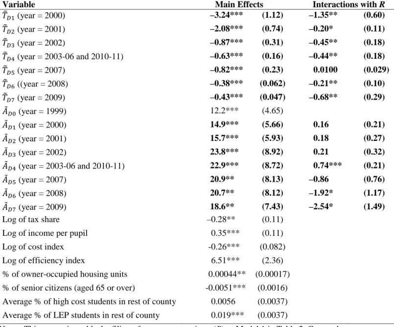
to the results of Hyashi, the correlation between this variable and R is large and positive (0.5). Table 4 presents results from a regression that adds interactions with R to Model 1 in Table 2. The review variable is defined as a deviation from the state-wide average, so that the other coefficients can be interpreted as effects at the average value of R. Adding these
interactions has little impact on the other coefficients in the regression (or on the hypothesis tests), but they indicate that the more reviews, the stronger the behavioral response to the STAR tax share. This effect is particularly large in 2000, when basic STAR was at its most salience. The interaction between the STAR tax share and R is not significant in 2007, when rebates were not in place at appeals time, but these interactions are significant in 2008 and 2009.
Flypaper Effects for State Aid
In Table 2, Model 1, the income elasticity of demand for S, θ, equals 0.23 and is significant. This θis in the range of previous studies. The aid flypaper effects, fA, are the coefficients of the A variables divided by the coefficient of income minus one. A larger fA
indicates a less salient local tax share, that is, a less salient discount in the value of $1 of aid. The pre-STAR fA is 34.9 (Table 3), which is higher than the estimates in the previous literature except for Eom et al. (2014), but lower than the STAR fA in any year, as in Hypothesis 4.27 In
addition, fA increases from 35.8 to 56.2 over the STAR years, which supports Hypothesis 5. The estimates of fA in the first two rebate years, 57.2 and 52.1, are not significantly different from the values in the nearby, non-rebate years, 56.2 (= f5). Because rebates are
excluded from the specification, we cannot reject the null hypothesis that the rebates have no impact on voter’s perceptions of the value of state aid, a result that is consistent with Hypothesis
6. The estimate of fA in the last rebate year, 42.8, is significantly lower than f5. This result is not
predicted by either salience or framing. Instead, we believe it reflects political and economic uncertainty in the spring of 2008, which led voters to expect aid cuts in the future and dampened their responses to aid in the May 2008 budget votes.28
These estimates of fA are larger than the maximum pre-STAR fP, 26.4, calculated above. However, these estimates of fA are considerably smaller than the maximum possible values of fP
with STAR. As shown above for the post-phase-in years, this maximum is 26.4 (the pre-STAR
fP) plus 88.6 (the change in fP when STAR exemptions are added), which equals 115.0—a number larger than the highest with-STAR fA. A more reasonable possibility is that two-thirds of
the estimated change in |µ| reflects an increase in |µC|. In this case, the STAR-induced change in the flypaper effect would be 29.6, for a total fP as high as 26.4 + 29.6 = 56, which is roughly equal to fA in the post-phase-in, non-rebate years.
Turning back to Table 4, we find that the interactions between the STAR-adjusted aid variables and R are generally not significant. The only significant interaction is for 2003-2006 plus 2010-2011, and it has an unexpected positive sign. Perhaps people who file reviews are more aware of state aid amounts than other people, which could boost their responsiveness to aid, but no more aware of the extent to which STAR lowers the value of aid to voters.
Conclusions
New York State’s STAR program provides a unique opportunity to study the impact of a tax’s administration on the behavioral responses to the tax. Property tax exemptions from STAR, which lower the price of local education, are delivered to homeowners as a line on their school property tax bill. For three years, however, these benefits were supplemented with a tax rebate that equaled a percentage of the savings from the exemption and arrived as a check in the mail.
We find signs of both salience and framing in the behavioral responses to these provisions. Our most striking result is that, despite their impact on voters’ tax shares, STAR rebates do not affect the demand for school quality because they arrive as unlabeled income. The importance of framing is supported both by the rejection of a model in which tax shares
incorporate rebates and by the finding that the non-response to rebates arises in all three rebate years, not just the year in which rebates were implemented after budget votes. The role of framing is also reinforced by our finding that rebates do not alter the flypaper effect attached to state educational aid, even though they alter voters’ tax shares.
Our strongest evidence for the importance of salience is the finding that voters’
behavioral responses to the STAR-based tax shares are largest when the STAR exemptions are most salient due both to publicity and to the magnitude of the tax savings. The importance of salience is also indicated by the larger behavioral response to the STAR tax share than to the less-salient standard tax share and by a smaller flypaper effect, that is, a more accurate recognition of voters’ net gains from state aid, when the STAR exemptions are most salient.
Finally, we make use of the Slutsky equation to show that behavioral responses to STAR tax shares reflect not only a substitution effect, but also an income effect, to which a flypaper effect might be attached. Our results are consistent with the view that this price-based flypaper effect is comparable in magnitude to the more familiar aid-based flypaper effect.
The key policy implication of our findings is that the outcomes of a property tax policy may depend on the way it is administered. In the case of STAR, the behavioral impacts of the STAR exemptions were magnified by the publicity surrounding their implementation, which gave them more salience. Moreover, the appearance of the STAR exemptions on a homeowner’s property tax bill framed them as a component of a household’s education budget, where they
directly affect education demand decisions. In contrast, the STAR rebates arrived in the mail, so they were framed as unlabeled income and had little or no impact on education demand.
Figure 1: STAR Application
Figure 2. Examples of Tentative Assessment Rolls, 2006 and 2008
Table 1. Summary Statistics (1999-2011)
Mean Std. Dev. Min Max
Dependent Variables
Performance index 75.8 11.6 29.2 98.2
Operating expenditures per pupil 15,766 4,003 9,164 74,269 STAR- and Rebate-Related Variables
Tax share 0.399 0.149 0.022 1.053 𝑇𝑇�𝐷𝐷1=1 0.891 0.042 0.751 0.984 𝑇𝑇�𝐷𝐷2=1 0.793 0.082 0.514 0.968 𝑇𝑇�𝐷𝐷3=1 0.698 0.121 0.287 0.949 𝑇𝑇�𝐷𝐷4=1 0.734 0.109 0.303 0.946 𝑇𝑇�𝐷𝐷5=1 0.664 0.139 0.168 0.922 𝑇𝑇�𝐷𝐷6=1 0.748 0.105 0.373 0.939 𝑇𝑇�𝐷𝐷7=1 0.753 0.102 .385 0.937 𝐴𝐴̃𝐷𝐷0=1 0.031 0.028 0.0003