In
September 2013
Estimating Fiscal Health of Cities: A
Methodological Framework for Developing
Countries
Simanti Bandyopadhyay
CENTER FORInternational Center for Public Policy Andrew Young School of Policy Studies Georgia State University
Atlanta, Georgia 30303 United States of America
Phone: (404) 651-1144 Fax: (404) 651-4449 Email: [email protected]
Internet: http://aysps.gsu.edu/isp/index.html
Copyright 2006, the Andrew Young School of Policy Studies, Georgia State University. No part of the material protected by this copyright notice may be reproduced or utilized in any form or by any means without prior written permission from the copyright owner.
International Center for Public Policy
Working Paper 13-19
Estimating Fiscal Health of Cities: A
Methodological Framework for Developing
Countries
Simanti Bandyopadhyay
September 2013
International Center for Public Policy
Andrew Young School of Policy Studies
The Andrew Young School of Policy Studies was established at Georgia State University with the objective of promoting excellence in the design, implementation, and evaluation of public policy. In addition to two academic departments (economics and public administration), the Andrew Young School houses seven leading research centers and policy programs, including the International Center for Public Policy.
The mission of the International Center for Public Policy is to provide academic and professional training, applied research, and technical assistance in support of sound public policy and sustainable economic growth in developing and transitional economies.
The International Center for Public Policy at the Andrew Young School of Policy Studies is recognized worldwide for its efforts in support of economic and public policy reforms through technical assistance and training around the world. This reputation has been built serving a diverse client base, including the World Bank, the U.S. Agency for International Development (USAID), the United Nations Development Programme (UNDP), finance ministries, government organizations, legislative bodies and private sector institutions.
The success of the International Center for Public Policy reflects the breadth and depth of the in-house technical expertise that the International Center for Public Policy can draw upon. The Andrew Young School's faculty are leading experts in economics and public policy and have authored books, published in major academic and technical journals, and have extensive experience in designing and implementing technical assistance and training programs. Andrew Young School faculty have been active in policy reform in over 40 countries around the world. Our technical assistance strategy is not to merely provide technical prescriptions for policy reform, but to engage in a collaborative effort with the host government and donor agency to identify and analyze the issues at hand, arrive at policy solutions and implement reforms.
The International Center for Public Policy specializes in four broad policy areas:
Fiscal policy, including tax reforms, public expenditure reviews, tax administration reform Fiscal decentralization, including fiscal decentralization reforms, design of intergovernmental
transfer systems, urban government finance
Budgeting and fiscal management, including local government budgeting, performance-based budgeting, capital budgeting, multi-year budgeting
Economic analysis and revenue forecasting, including micro-simulation, time series forecasting,
For more information about our technical assistance activities and training programs, please visit our website at http://aysps.gsu.edu/isp/index.html or contact us by email at [email protected].
* The author would like to thank Aishna Sharma and Sujana Kabiraj for their assistance at different stages of the work. Sincere thanks are due to Debraj Bagchi for his comments and suggestions. However the usual disclaimer applies.
1
Estimating Fiscal Health of Cities: A
Methodological Framework for Developing
Countries*
Simanti Bandyopadhyay National Institute of Public Finance and Policy
Abstract
The main objective of the paper is to propose a framework in which fiscal health conditions can be assessed and the main determinants affecting fiscal health can be identified, inspite of severe data constraints. The paper draws on big urban agglomerations in India as well as smaller cities as a sample and attempts to identify the difference, if any, in the main determinants for variations in fiscal health conditions across different size classes of cities. To compensate for the lack of statistical rigor in the estimations of expenditure needs and revenue capacities, we propose a framework which analyses the ratio of expenditure needs to revenue capacity by fitting an econometric model. It is a two-step method, in the first stage we estimate the expenditure need and revenue capacity separately by simple methods discussed above. In the second stage we take the ratio of expenditure need and revenue capacity as an indicator of financial performance of a ULB and fit an econometric model to explain the performance of ULBs on the basis of factors which are likely to affect the performance of the ULBs. We find that the role of the higher tiers of the government is important in bigger and smaller size class of cities in their financial management. However, for bigger cities we find that the own source revenues can also play an important role in bringing down the fiscal ratio. In the smaller ULBs the role of the demand indicators is not that prominent but the cost indicators play a relatively prominent role. In case of bigger agglomerations, the demand indicators are more prominent than the cost indicators.
1. Introduction
Assessing fiscal health of urban local bodies has always been a challenge for researchers. Formulating a methodology is harder in case of the developing countries particularly due to severe data constraints. The methodologies that have been formulated and applied in the literature in case of developed countriesare not appropriate for developing countries. As a result of which there is a lack of literature analysing fiscal issues at the city level for developing countries which have followed a rigorous methodology.The main objective of the paper is to propose a framework in which fiscal health conditions can be assessed and the main determinants affecting fiscal health can be identified, inspite of severe data constraints. The paper draws on big urban agglomerations in India as well as smaller cities as a sample and attempts to identify the difference, if any, in the main determinants for variations in fiscal health conditions across different size classes of cities.
The paper is organised as follows. Section 2 gives a brief literature review on the methodologies on assessing the fiscal health of cities; section 3 elaborates on the difficulties in applications of these methodologies in general and also with special reference to Indian cities and spells out the modifications needed in the existing framework to assess fiscal health in Indian cities ; section 4 gives an application of the modified framework proposed in section 3 for Indian cities; section 5 concludes the paper.
2. Literature Review
One way to assess the fiscal conditions of governments is by comparing the gap between expenditure needs and revenue-raising capacity. This gap is generally referred to as a need-capacity or fiscal gap. The minimum amount of money needed to provide basic acceptable levels of public services for those functions assigned to the urban local government is referred to as the expenditure need of the local government. `The resources the government is expected to raise from local sources at a “normal” or “standard” rate of revenue effort is referred to as the revenue capacity.
The expenditure need estimations depend on services to be provided by the local government and the costs associated to provide these services. Given the responsibilities of the local governments to provide a set of services, the crucial step in estimating expenditure need is the estimation of costs (Reschovsky 2007). One way to estimate a cost function of a service is to derive it from the production function which requires data on outputs of public services. Quantifying a public output is as difficult as empirically measuring it. Also, there is an element of simultaneity involved in estimating these functions empirically. Though two stage estimation methods are proposed in the literature to tackle this problem, often the data requirements to carry out such procedures are not fulfilled.
Cost functions for primary and secondary education in the United States have been estimated (Duncombe and Yinger 2000; Reschovsky and Imazeki 2003; Imazeki and Reschovsky 2005). For estimating the expenditure need the coefficients of the estimated cost function can be used to construct a cost index which is the summary measure and can be used to determine the expenditure requirements once the level of service provision is specified. Expenditure equations in reduced form are also estimated instead of cost functions to avoid the statistical complexity and daunting data requirements of cost function estimations. The expenditure functions can be explained by a set of cost, demand and resource factors. Expenditure equations also can be used to derive cost indices by predicting the local government’s spending with average values for the demand and resource variables but actual values of the cost variables from the estimated expenditure equations and then dividing each of these predicted values by the expenditure of the local government with average costs. Bradbury et al (1984) use this methodology using data for Massachusetts.
There are two major approaches to measure revenue capacity: The Representative tax system approach and Regression or stochastic approach. The Representative Tax Approach involves three major steps, first, for each tax, an appropriate base has to be identified. This base should not be the base which is recorded in official tax statistics, rather it should be the base that can be taken to be representative of relative taxable capacity. Second, a set of representative tax rate
which can be constituted as representative tax system need to be generated. This representative rate of the tax may be derived as the average of the effective rates of that tax, where the effective rates are defined as the ratio of actual collection to the potential base.
Third, the average effective rate (AER) for each source can be calculated as a weighted average of the effective rates of all the sources, weights being the share of each source. The product of AER and the potential base of a tax will indicate the revenue which the concerned ULB could raise from that source if its average level of potential is used.
In Regression or stochastic approach the variation of tax ratio can be explained by a regression analysis where tax ratio is taken as the dependent variable and indicators of tax capacity and tax effort factors as independent variables. The actual tax ratio depends on the ability of the people to pay taxes, the ability of the administration to collect taxes and the willingness of the government to tax. The factors affecting first two components are termed as tax capacity factors and the factors affecting the third component are tax effort factors.
Alternatively, an attempt can be made to quantify and isolate the tax capacity factors on the tax ratio, so that the measure of the tax effort of the government will be derived on the basis of residuals. The average degree of the relationship between the tax ratio and the factors identified to affect taxable capacity may be derived through multiple regression analysis. The difference between the actual tax ratio in a ULB and that estimated for it on the basis of tax capacity equation would be the unexplained variance component and may be attributed to tax efforts.
Tax effort can be measured in one of the two ways: some expression of the residual variance can be taken as the measure of tax effort .Alternatively the estimated tax ratio can be taken to represent the relative taxable capacity. Thus a comparison of the actual tax ratio for a ULB with its estimated ratio will show the ULB’s tax effort. As the overall tax ratio is employed in this method, this method is called the aggregate regression method.
3. A Modified Methodological Framework
This paper attempts to develop a framework for assessing fiscal health for cities in the developing world where data is not available to the degree of disaggregation required for assessment of fiscal health by the methodologies proposed in the literature (Bandyopadhyay and Rao 2009, Krueathep 2010). Within the existing methodological framework we would like to bring in some modifications so that we can use the data available to estimate the fiscal gap.
There are two main components in measuring fiscal gap in a city. The expenditure needs component can be estimated by econometric methods for which city level data on consumption of local services are needed. Also, we need city level norms for these services. These requirements cannot be fulfilled in case of Indian cities. Also, apart from the expenditure on services, there are expenditures which cannot be categorized and thus cannot be specified to have norms. So it is very difficult to quantify the ideal level for a part of the expenditures which is heterogeneous in nature, but constitutes a considerable share in the expenditure of a ULB (Bandyopadhyay 2011, Bandyopadhyay and Rao, 2009, NIPFP (2007a, 2007b, 2007c, 2007d, 2008a).
For all these difficulties we have estimated expenditure needs from expert opinion. In India we have expert groups specifying minimum acceptable physical levels of these services according to city size classes to provide as physical norms. Corresponding to these physical norms, ideal levels of expenditures as financial norms for these services are also estimated. We have used the latest HPEC (2011) norms for Indian cities in this paper. We have taken five major services viz water supply, sewerage/sanitation, street lighting, roads and solid waste management and have estimated the financial requirements in per capita terms on these services. We sum up the financial norms for all these services and estimate the expenditure need on these services for the ULB.
The standard methodologies estimating the revenue capacities are very demanding as far as data requirements are concerned in general. Estimating the representative tax base is extremely difficult in the absence of data required to the level
of disaggregation and involves some amount of subjectivity. The applicability of these methods in case of Indian cities is restricted in particular as the data on proxies for urban tax base, for instance incomes of cities, are not available in India. The problem with regression approach is the conceptualization of the residuals as a measure of tax effort. Also, estimating a model identifying factors affecting taxable capacity becomes difficult as it involves elements of simultaneity.
To overcome these methodological problems we have estimated revenue capacity by a simple procedure. We propose to estimate the city level incomes from the data on district level domestic products. We take the ratio of own revenue to GCP and propose a higher own revenue to GCP ratio as the desired rate at which revenues can be generated and also which are politically feasible (Bandyopadhyay 2011, Bandyopadhyay and Rao, 2009).
To compensate for the lack of statistical rigor in the estimations of expenditure needs and revenue capacities, we propose a framework which analyses the ratio of expenditure needs to revenue capacity by fitting an econometric model. It is a two step method, in the first stage we estimate the expenditure need and revenue capacity separately by simple methods discussed above. In the second stage we take the ratio of expenditure need and revenue capacity as an indicator of financial performance of a ULB and fit an econometric model to explain the performance of ULBs on the basis of factors which are likely to affect the performance of the ULBs. We categorise the explanatory variables for the model into five categories viz. resource, demand, infrastructure, service and cost. The resource variables are different sources of municipal revenues, the demand variables would affect the performance from the demand side of the inhabitants of the city, infrastructure indicators are those which are combined outcomes of the efforts of the urban local bodies and the upper tiers of the government or PPP like electricity provision, banks etc, service indicators give the state of local services in the ULBs, cost indicators affect the performance through the cost of provision of local services. The categorization is elaborated in Bandyopadhyay (2011).
Models are generated with three sets of financial ratios as the dependent variable viz. Capital expenditure need to revenue capacity model (taking only capital
expenditure needs) and Revenue expenditure need to revenue capacity model (taking only revenue expenditure needs), Total expenditure need to revenue capacity (taking both capital and revenue expenditure needs together). The magnitudes of ratios give an indication of what proportion of the expenditure needs can be financed once the revenue capacity is realized. A value greater than 1 would indicate that expenditure need cannot be covered even if the revenue capacity is realized in the ULB.
The main advantage of this methodology is that we can not only estimate the expenditure needs and revenue capacities but also get an idea about the main determinants of the financial performance of the ULBs. This methodology is particularly helpful in assessing the fiscal health of cities in developing countries because it is more flexible and thus less demanding as far as data requirement is concerned. The approach is an indirect one but can bring out interesting insights explaining performances of cities. In the following section we would discuss a case study on Indian cities using this methodology.
4. Fiscal Health of Indian Cities
We take a sample of metropolitan cities and smaller cities from comparatively backward areas of India to attempt an analysis of fiscal health. Our sample constitutes of five big agglomerations in India viz Delhi, Kolkata, Chennai, Hyderabad and Pune and the urban local bodies of the state of Jharkhand and eight adjacent districts of West Bengal which share their borders with Jharkhand. The details of the metropolitan cities are given in Bandyopadhyay and Rao (2009) and those of the smaller ULBs in Bandyopadhyay and Bohra (2010) and Bandyopadhyay (2011).
As we have mentioned in the previous section, the dependent variable is the financial performance indicator of a ULB expressed as a ratio of the expenditure need to revenue capacity. The categories of explanatory variables are summarized in table 1. The data on resource indicators are collected in course of primary surveys from the budgets of the ULBs whereas the variables in the other categories are collected from Census of India. The models are fitted separately for cities in bigger urban agglomerations and smaller ULBs. We have three models for each class of cities.
Table 1: Category wise Explanatory Variables for Performance of ULBs
Category Variables
Resource Indicators Property Tax, Tax, Non Tax Revenue, Transfers
Demand Indicators Households having No Assets, Households Availing Banking Facilities and Literacy
Infrastructure Indicators Electricity per 1000 population, Domestic and Non Domestic Connections per 1000 population, Non domestic Connections to total connections(%), Banks per Sq Km
Service Indicators Roads per 1000 population, Street lights per 1000 population, Households having water within premises (%), Households having tap water(%),Households having closed surface drainage(%), Toilets per 1000 population Cost Indicators Population, Number of Households, Household Size,
Area(sq km),Density
The principle in which the model works is very simple. All the explanatory variables are likely to affect both the expenditure needs and the revenue capacity separately. Some effects are direct while some work through indirect chains. The relative strength of the two would determine the effect of the determinants on the financial ratios as performance indicators of ULBs. The empirical justification would come by splitting the two effects to analyse the resulting impact.
We take the resource category to explain the idea. The resource variables are likely to affect the revenue capacity as higher values of these variables would be associated with higher values of revenue capacities. The own revenue components would have an effect through own revenue to GCP ratio whereas the transfers would have a direct impact. On the other hand these variables would have an indirect impact on expenditure needs. A higher own revenues would mean that the inhabitants are capable of giving higher taxes and also the jurisdictions have a better administrative efficiency. A higher tax and non tax-paying inhabitants would likely to put pressure on the government to provide higher and better levels of services, thus having a positive
impact on expenditure needs. The effect of a resource variable on the financial ratio would be determined by the relative strengths of the two effects. This is an empirical question. Similarly, all the categories of explanatory variables would have some impact from the demand side and some from the supply side on the two components of the ratio and end result would determine the sign and magnitude of the regression coefficients which is an empirical question.
In what follows we would analyse and interpret the results of the models fitted in the paper.
Smaller ULBs models
A Sample size of 88 ULBs includes all ULBs in the state of Jharkhand and those located in eight adjacent districts of the state of West Bengal. All the models are log-log models. We attempt three sets of regressions, with the total expenditure needs, capital expenditure needs and revenue expenditure needs with the same set of explanatory variables. The descriptive statistics and the results are summarized in Appendix 1. Model 1 Total expenditure need to revenue capacity model
We study the determinants of the total expenditure needs to revenue capacity ratio. We find that higher the grants from the higher tier government, higher the revenue capacity with little or no effect on expenditure needs. In our sample of smaller cities, we find that intergovernmental transfers in the form of grants play a positive role in bringing down the fiscal gap.
Service indicator like proportion of households having water within premises has a positive role to play in explaining the performance of a city. A ULB which has higher service provision and infrastructure provision has already met the minimum basic standards and has better living conditions and hence there will be less pressure on the expenditure side. So, better service provision at the local level can lead to a better fiscal health of cities.
Also better infrastructure provision like electricity which is done at the state level or with PPP can lead to a better fiscal health of cities. This is indicative to the fact that
higher level participation is needed for better performance in fiscal management at the local level.
A ULB which has a higher population growth is the one which can attract people for economic and political reasons in its jurisdiction. The immediate effect would be a pressure on the government in terms of service provision. It can also generate a greater amount of own revenues in the form of taxes, fees and charges. In our sample of cities we find the pressure on expenditure needs is offset by the rise in revenue capacity. This leads to a better fiscal health.
However, a higher per capita total tax revenue is associated with a higher ratio. In these cities raising taxes would not necessarily lower the fiscal gap.
Higher density would have a negative impact on fiscal health in our sample. It can cause the revenue capacity to rise because of more potential contributors to revenues in densely populated cities. Whether expenditure needs would rise would depend on the nature of services provided and the stage of operation for the service as due to economies of scale some services can be provided at a lesser cost in more densely populated areas. In our sample of cities we find population density to have an adverse impact on fiscal health. ULBs with higher population densities are unlikely to perform better in terms of fiscal health.
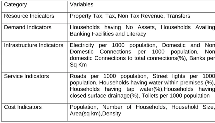
Model 2. Capital expenditure need to Revenue capacity model
We study the determinants of capital expenditure needs to revenue capacity model separately. We find that Transfers and grants from the higher tier government raise the revenue capacity and reduce the ratio.
. Service indicators like households having water within premises (%) and households having tap water (%) and infrastructure indicator like number of domestic and non domestic electricity connections per 1000 population have a negative impact on the ratio like the total expenditure needs model..
Non tax revenues play a negative impact on fiscal health defined in terms of capital expenditures.
Area and population density also affect the ratio adversely. Higher the density and area, higher will be pressure on the local government expenditure. Higher area and density can also be interpreted as higher potential for revenues. In our sample of cities the expenditure effect dominates causing a higher ratio to be associated with a higher Area and density.
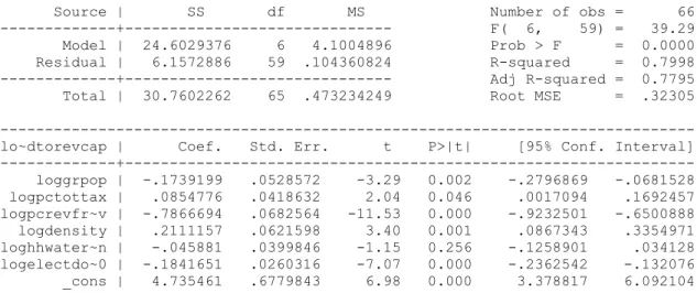
Model 3 Revenue expenditure need to Revenue capacity model
We study the determinants of Revenue expenditure need to revenue capacity ratio model separately. We find that higher the transfer and grants from the higher tier government, better the fiscal health indicators in terms of revenue expenditure needs.
Service indicators like Proportion of households with water sources within premises would have a positive impact on the fiscal health indicator. A ULB with a higher proportion of households with water sources within premises would have a lower revenue expenditure need to revenue capacity ratio in our sample.
A higher Population growth can lead to a better fiscal health in our sample of smaller ULBs.
A higher Per capita Total tax revenue is associated with higher financial ratios of ULBs in our model.
Also, cost indicators like Area, Population Density have an adverse impact on fiscal health.
We find that across the models the same significant variables have the same signs. It can be noted that the variables which affect the revenue expenditure need to revenue capacity and capital expenditure need to revenue capacity are the ones which also affect the total expenditure need to revenue capacity model. However, there are exceptions. In case of revenue and capital models, area is a significant variable, but it is not a significant variable in the total model. Similarly, non tax revenue is a significant
variable in the capital expenditure need model but not in the total model. Also, number of domestic and non domestic electricity connections per 1000 population is significant is capital and total model but not in the revenue model. Proportion of households with tap water connections is significant in the capital model but not in any other model. It is also to be noted that none of the demand category indicators are significant in any of the models for smaller ULBs.
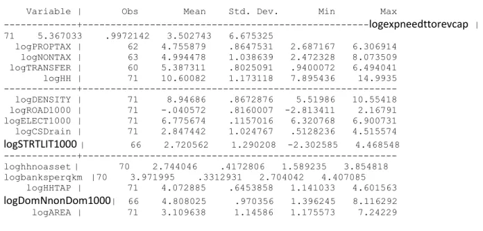
Agglomerations Models
A Sample of 71 ULBs are considered from five major urban agglomerations in India, viz. Delhi, Kolkata, Chennai, Hyderabad and Pune. We attempt three sets of regressions, with the total expenditure needs, capital expenditure needs and revenue expenditure needs with the same set of explanatory variables. The descriptive statistics and the results are summarized in Appendix 2.
Model 1 Total expenditure need to revenue capacity model
We study the determinants of the total expenditure needs to revenue capacity ratio. We find that three components of the resource category indicators viz.Per capita property tax, Per capita nontax, Per capita assigned revenue are significant and can affect fiscal health in a positive way. In the agglomerations model, bigger cities gain both from own sources and transfers to lower the financial ratio. As property tax, nontax collection and assigned revenue rise, the effect on revenue capacity of a ULB dominates as a result of which ULBs having higher revenue collections in these categories are the ones having better fiscal health. So a better performance in the own source components can assure a better fiscal health in the bigger cities. Assigned revenues are also a part which is generated through activities in a ULB but goes to the state and comes back as a share to the ULBs. So in bigger ULBs a better performance in revenue collections can ensure better fiscal health.
We also find that Number of Electricity connections per 1000 population can affect fiscal health in a positive way. Better infrastructure conditions are provided by the upper tiers of the government which in our sample of bigger cities can cause a better fiscal health of the local government.
We also find that demand indicators like asset possession of households can affect the fiscal health in a positive way. Proportion of households having no assets is significant with a positive sign. An increase in the households with no asset is indicative of low development and low standard of living of the people residing in a ULB. This hampers the revenue and thus revenue capacity falls causing the ratio to rise. This also indicates less pressure on the expenditure needs as people with lower standard of living would likely to put lesser pressure on the local government for provision of quality services. In our sample of bigger cities, the revenue capacity effect seems to dominate. We can infer that the higher the proportion of people having below average standard of living, lower would be the performance in terms of fiscal health.
However, demand indicator like Proportion of households availing banking facilities would have an adverse impact on the fiscal health ratio in our sample of cities.
We also find that Number of toilets per 1000 population can affect the fiscal health in an adverse way. In our sample of cities the expenditure effect seem to dominate and we find that the ULBs having higher proportions of people with better standard of living do not perform better in terms of fiscal health indicators.
Model 2 Capital expenditure need to revenue capacity model
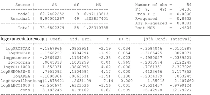
We study the determinants of the capital expenditure needs to revenue capacity ratio for the agglomeration cities. We find that Per capita property tax, per capita non tax revenue, per capita assigned revenue can play a positive role on fiscal health of cities. As property tax, nontax collection and assigned revenue rise, revenue capacity of a ULB increases and the effect dominates that on the capital expenditure needs. This reduces the ratio.
We also find that Number of Electricity connections per 1000 population can affect fiscal health in a positive way.
The asset possession of households reflected in Proportion of households having no asset is significant and have a positive sign. An increase in the households with no asset is indicative of low development and low standard of living of the people residing
in a ULB. This hampers the revenue and thus revenue capacity falls causing the ratio to rise. However, demand indicator like Proportion of households availing banking facilities would have an adverse impact on the fiscal health ratio in our sample of cities.
Service indicators like Number of toilets per 1000 population is significant but have a positive sign.
Cost indicator like Area is significant and have a positive sign in explaining the capital expenditure needs to revenue capacity model.. Higher area can lead to higher tax collection and thus increases the revenue capacity. Also, a higher coverage of area can have a positive or negative impact on expenditure on services depending upon the nature of services and the stage of operation. In our sample of cities size of the ULB is not indicative of a better fiscal health which means neither the revenue potential advantage is utilized nor are there economies of scale advantages reducing expenditure needs.
Model 3 Revenue expenditure need to revenue capacity model
We study the determinants of Revenue expenditure need to revenue capacity model. We find that per capita property tax revenue, per capita nontax revenue, per capita assigned revenue can affect the revenue expenditure need to revenue capacity ratio in a positive way. These are all a source of increase in revenue capacity. As these variables increase, the revenue capacity rises and this reduces the ratio.
We also find that Number of Electricity connections per 1000 population has a positive effect on fiscal health defined in terms of revenue expenditure needs in our sample of agglomeration cities. We also find that the indicator of asset possession of households can have a positive impact on the fiscal health of these cities.
However, demand indicator like Proportion of households availing banking facilities would have an adverse impact on the fiscal health ratio defined in terms of revenue expenditure needs in our sample of cities.
We also find that Number of toilets per 1000 population can affect the fiscal health ratio defined in terms of revenue expenditure needs in a negative way
It can be seen that the total model is a combination of revenue and capital expenditure need model. There is not much difference between the significant variables across the models. However, non tax is significant in only total expenditure need and revenue expenditure need model and not the capital expenditure need model at 5 per cent level of significance. The resource variables in the total model behave in the same way as the capital model. None of the cost variables are significant except Area in the capital model.
A broad comparison between smaller ULB models (Jharkhand and West Bengal) and bigger ULB models (5 UAs) by considering only the total expenditure need model gives a few points of similarity between the models. Transfers is a significant common resource variable in both the models carrying a negative sign. For bigger agglomerations, it is the assigned revenue components and not the grant component which can help reducing the fiscal gap ratio. Also, Number of electricity connections per 1000 population has a negative effect on the ratio in both the models. Transfers and infrastructure like electricity involve the role of the upper tiers of the government. This implies that better financial performance of the ULBs, irrespective of size, can be explained by a better performance of the upper tiers of the government in providing infrastructure or releasing grants,
There are a few points of differences too. Whereas in the bigger ULB model, cities with better service indicators have higher values of expenditure need to revenue capacity ratio, the cities with better service indicators would have lower expenditure need to revenue capacity ratios in smaller ULB model. Also, in the smaller ULB model the total tax is significant, in case of bigger ULB model, it is not the total tax but property tax and non tax both are significant separately. In fact, in smaller ULBs a higher tax level cannot bring down the gap but widens it, whereas in the bigger ULBs higher levels of the own revenue components can bring down the gap. Another interesting finding is that none of the demand variables has significant effect on the ratio in case of smaller ULB models. In contrast, demand variables (households availing banking facilities and households having none of the assets) are significant in case of bigger ULB model.
5. Conclusion
The paper offers an alternative framework for assessing fiscal health of urban local bodies in developing countries. The methodologies proposed so far in the literature to estimate the fiscal gaps are not always suitable in case of developing countries due to non availability of data to the disaggregation levels required. The present framework proposed derives the expenditure needs and revenue capacities using simple methods but attempts an econometric analysis of the fiscal gaps by fitting a model which can explain the differences in fiscal gaps across cities through socio demographic, cost, demand, resource, infrastructure and service indicators of these cities. This way the data requirements in estimating the expenditure needs and revenue capacities separately are not that demanding but in the second stage we can explain the differences in fiscal gaps from available data which can give us meaningful insights.
The paper attempts an application with a case study with cities of different size classes in India. We find that the role of the higher tiers of the government is equally important in bigger and smaller size class of cities in their financial management. However, for bigger cities we find that the own source revenues can also play an important role in bringing down the fiscal ratio. In the smaller ULBs the role of the demand indicators is not that prominent but the cost indicators play a relatively prominent role. In case of bigger agglomerations, the demand indicators are more prominent than the cost indicators.
A few limitations of the study can be spelt out in the end. The categorization of the explanatory variables might have some overlap across categories. Some of the cost or infrastructure indicators can play a role in determining the demand for urban services. This is reflected in the regression results which we analyse and interpret intuitively but quantifying the impact as specific to each category might not be possible. However, we have followed a conceptual framework which is clear in terms of defining these variables. Our analysis is still constrained by availability of data because of which we cannot attempt any other model apart from simple OLS. With limited data this paper develops a framework that can throw some light on the fiscal performance of the ULBs in developing countries.
References
Bandyopadhyay S, (2011); ‘Finances of Urban Local Bodies in Jharkhand: Some Issues and Comparisons’, International Studies Program Working Paper 11-13, Andrew Young School of Policy Studies, Georgia State University, Atlanta, USA, May 2011.
Bandyopadhyay. S, and Bohra O P (2010): Functions and Finances of Urban Local Bodies in Jharkhand, Draft Report submitted to Governm ent of Jharkhand, National Institute of Public Finance and Policy, New Delhi.
Bandyopadhyay. S and Rao M.G (2009): Fiscal Health of Selected Indian Cities’, Policy Research Working Paper No: 4863, The World Bank, World Bank Institute, Poverty Reduction and Economic Management Division, Washington DC, March 2009.
Bradbury, K, L.,Helen, F. Ladd, M Perrault, A Reschovsky, and J Yinger. 1984. "State Aid to Offset Fiscal Disparities Across Communities," National Tax Journal 37, no. 2, (June): 151-170.
Duncombe,W and J. Yinger 2000.“Financing Higher Student Performance Standards: The Case of New York State.” Economics of Education Review 19 (4): 363–86.
Imazeki, J, and A Reschovsky. 2005. “Assessing the Use of Econometric Analysis in Estimating the Costs of eeting State Education Accountability Standards: Lessons from Texas.” Peabody Journal of Education 80 (3): 96–125.
Krueathep W (2010). Bad Luck Or Bad Budgeting A Comparative Analysis Of Municipal Fiscal Conditions In Thailand, PhD Thesis, Graduate School-Newark, Rutgers, The State University of New Jersey, School of Public Affairs and Administration.
NIPFP (2007a) Improving the Fiscal Health of Indian Cities: A Pilot Study of Kolkata, NIPFP, New Delhi, Draft Report, Submitted to World Bank.
NIPFP (2007b) Improving the Fiscal Health of Indian Cities: A Pilot Study of Delhi, NIPFP, New Delhi, Draft Report ,Submitted to World Bank.
NIPFP (2007c) Improving the Fiscal Health of Indian Cities: A Pilot Study of Pune, NIPFP, New Delhi, Draft Report, Submitted to World Bank.
NIPFP (2007d) Improving the Fiscal Health of Indian Cities: A Pilot Study of Hyderabad, NIPFP, New Delhi, Draft Report , Submitted to World Bank.
NIPFP (2008 a) Improving the Fiscal Health of Indian Cities: A Pilot Study of Chennai, NIPFP, New Delhi, Draft Report, Submitted to World Bank.
NIPFP (2008 b) Improving the Fiscal Health of Indian Cities: A Synthesis of Pilot Studies, NIPFP, New Delhi, Draft Report, Submitted to World Bank.
NIPFP (2009): Urban Property Tax Potential In India, Submitted to Thirteenth Finance Commission, India.
HPEC (2011) Report on Indian Urban Infrastructure and Services, Government of India.
Reschovsky. A (2007) Compensating Local Governments for Differences in Expenditure Needs in a Horizontal Fiscal Equalization Program, Chapter 14 in The Theory and Practice of Intergovernmental Fiscal Transfers, edited by Robin Boadway and Anwar Shah, Washington, DC, The World Bank, 2007: 397-424.
Reschovsky, A, and J Imazeki. 2003. “Let No Child Be Left Behind: Determining the Cost of Improved Student Performance.” Public Finance Review 31 (3): 263–90.
Appendix 1 Smaller ULBs models
Table A 1 Summary Statistics
Variable | Obs Mean Std. Dev. Min Max
---+--- logpop | 88 10.95548 .9506024 8.823501 13.64957 loggrpop | 85 3.262568 .782116 1.386294 6.148468 loghh | 86 9.200686 .9621989 7.094235 11.88364 logarea | 88 2.680783 .8587232 1.172482 5.177223 logpcproptax | 69 2.843262 1.292715 -.5798185 6.120297 ---+--- logpcothertax | 68 1.820533 1.624707 -2.995732 4.60517 logpctottax | 72 3.247489 1.25295 -.3710637 6.196444 logpcnontax | 71 2.763857 1.772648 -2.65926 5.463832 logpcownrev | 73 3.903768 1.210573 -.2744369 6.393591 logpctransfer | 72 5.234513 .8428414 1.922788 7.907968 ---+--- logpctotrev | 75 5.479287 .979284 1.922788 7.914621 logdensity | 86 8.227163 .805521 6.709329 9.937987 logroadper1000 | 70 .3935277 .6520125 -.2629639 4.007333 logliteracy | 82 4.203502 .1132699 3.637586 4.394449 loghhtap | 87 3.271534 .980384 0 4.584968 ---+--- logbanksper100sqkm | 86 3.717921 .8535008 1.098612 5.717028 loghhwaterwithin | 86 2.278777 1.191427 0 4.127134 logcsdrain | 88 2.160353 .8139805 0 4.007333 logelectper1000| 88 6.392644 .3094466 5.062595 6.860664 logtoiletper1000| 88 6.400831 .3375505 4.682131 6.820016 ---+--- loghhnoasset | 66 3.261761 .3383825 2.397895 4.007333 logexpneedctorevcap | 75 -.2633242 1.272061 -3.723553 1.564821 logexpneedrtorevcap | 75 .2194891 .6338504 -2.249063 1.41049 lognondomtototelect | 86 -1.271436 .713286 -6.216606 -.0730519 loghhsize | 86 1.740954 .0983636 1.361738 2.007086 ---+--- logexpneedtorevcap| 75 .787879 .8147802 -2.042947 2.167597
Model 1 Total Expenditure need to revenue capacity model: Table A2 Regression Reults
Source | SS df MS Number of obs = 66 ---+--- F( 6, 59) = 39.29 Model | 24.6029376 6 4.1004896 Prob > F = 0.0000 Residual | 6.1572886 59 .104360824 R-squared = 0.7998 ---+--- Adj R-squared = 0.7795 Total | 30.7602262 65 .473234249 Root MSE = .32305 --- lo~dtorevcap | Coef. Std. Err. t P>|t| [95% Conf. Interval] ---+--- loggrpop | -.1739199 .0528572 -3.29 0.002 -.2796869 -.0681528 logpctottax | .0854776 .0418632 2.04 0.046 .0017094 .1692457 logpcrevfr~v | -.7866694 .0682564 -11.53 0.000 -.9232501 -.6500888 logdensity | .2111157 .0621598 3.40 0.001 .0867343 .3354971 loghhwater~n | -.045881 .0399846 -1.15 0.256 -.1258901 .034128 logelectdo~0 | -.1841651 .0260316 -7.07 0.000 -.2362542 -.132076 _cons | 4.735461 .6779843 6.98 0.000 3.378817 6.092104 ---
Model 2 Capital expenditure need to revenue capacity model: Table A3 Regression Results
Source | SS df MS Number of obs = 67
---+--- F( 7, 59) = 59.69 Model | 77.8384489 7 11.1197784 Prob > F = 0.0000 Residual | 10.9907035 59 .18628311 R-squared = 0.8763 ---+--- --- Adj R-squared = 0.8616 Total | 88.8291524 66 1.34589625 Root MSE = .43161 --- lo~ctorevcap | Coef. Std. Err. t P>|t| [95% Conf. Interval] ---+--- logpcnontax | .1184747 .0378699 3.13 0.003 .0426973 .1942521 logarea | .2042933 .0829394 2.46 0.017 .0383319 .3702547 loghhtap | .4686725 .0858685 5.46 0.000 .2968501 .640495 logpcrevfr~v | -.6160993 .0928023 -6.64 0.000 -.8017963 -.4304023 logdensity | .4848385 .0957527 5.06 0.000 .2932377 .6764393 loghhwater~n | -.3606339 .0778723 -4.63 0.000 -.5164561 -.2048117 logelectdo~0 | -.3115579 .034053 -9.15 0.000 -.3796977 -.2434181 _cons | -.7059695 1.196781 -0.59 0.558 -3.100722 1.688783
Model 3 Revenue expenditure need to revenue capacity model: Table A 4 Regression results
Source | SS df MS Number of obs = 66 ---+--- F( 6, 59) = 32.94 Model | 13.8988369 6 2.31647282 Prob > F = 0.0000 Residual | 4.14904795 59 .070322847 R-squared = 0.7701 ---+--- Adj R-squared = 0.7467 Total | 18.0478849 65 .277659767 Root MSE = .26518 --- lo~rtorevcap | Coef. Std. Err. t P>|t| [95% Conf. Interval] ---+--- logpctottax | .0955929 .0272853 3.50 0.001 .0409951 .1501907 loggrpop | -.109789 .0442319 -2.48 0.016 -.1982968 -.0212812 logarea | .114944 .0530166 2.17 0.034 .0088582 .2210299 logpcrevfr~v | -.6472934 .0606788 -10.67 0.000 -.7687115 -.5258754 logdensity | .2081177 .0616096 3.38 0.001 .0848372 .3313983 loghhwater~n | -.0767681 .0368665 -2.08 0.042 -.1505377 -.0029984 _cons | 1.810751 .7284178 2.49 0.016 .3531906 3.268312
Appendix 2 Agglomerations models
Table A5 Summary Statistics
Variable | Obs Mean Std. Dev. Min Max
---+---logexpneedttorevcap | 71 5.367033 .9972142 3.502743 6.675325 logPROPTAX | 62 4.755879 .8647531 2.687167 6.306914 logNONTAX | 63 4.994478 1.038639 2.472328 8.073509 logTRANSFER | 60 5.387311 .8025091 .9400072 6.494041 logHH | 71 10.60082 1.173118 7.895436 14.9935 ---+--- logDENSITY | 71 8.94686 .8672876 5.51986 10.55418 logROAD1000 | 71 -.040572 .8160007 -2.813411 2.16791 logELECT1000 | 71 6.775674 .1157016 6.320768 6.900731 logCSDrain | 71 2.847442 1.024767 .5128236 4.515574 logSTRTLIT1000 | 66 2.720562 1.290208 -2.302585 4.468548 ---+--- loghhnoasset| 70 2.744046 .4172806 1.589235 3.854818 logbanksperqkm |70 3.971995 .3312931 2.704042 4.407085 logHHTAP | 71 4.072885 .6453858 1.141033 4.601563 logDomNnonDom1000| 66 4.808025 .970356 1.396245 8.116292 logAREA | 71 3.109638 1.14586 1.175573 7.24229
Model 1 Total expenditure need to revenue capacity model:
Table A 6 Regression Results
Source | SS df MS Number of obs = 59
---+--- F( 8, 50) = 38.68 Model | 47.1048026 8 5.88810032 Prob > F = 0.0000 Residual | 7.61093867 50 .152218773 R-squared = 0.8609 ---+--- Adj R-squared = 0.8386 Total | 54.7157412 58 .943374849 Root MSE = .39015
logexpneedttorevcap | Coef. Std. Err. t P>|t| [95% Conf. Interval] ---+--- logPROPTAX | -.1709645 .0721881 -2.37 0.022 -.3159586 -.0259705 logNONTAX | -.1605345 .0686512 -2.34 0.023 -.2984244 -.0226446 logTRANSFER | -.242977 .0738452 -3.29 0.002 -.3912995 -.0946545 logTOIL1000 | 1.512727 .329232 4.59 0.000 .8514453 2.174009 logHHNOASS~S | .6974756 .1643095 4.24 0.000 .3674503 1.027501 logAREA | -.1042181 .0523371 -1.99 0.052 -.2093402 .0009041 logHHAvail~c | 1.662951 .209093 7.95 0.000 1.242975 2.082927 logELECT1000 | -2.041463 .5332599 -3.83 0.000 -3.112547 -.970379 _cons | 3.709285 4.025003 0.92 0.361 -4.375172 11.79374
---Model 2 Capital expenditure need to revenue capacity model: Table A 7 Regression Results
Source | SS df MS Number of obs = 59 ---+--- F( 9, 49) = 34.36 Model | 62.7402252 9 6.97113613 Prob > F = 0.0000 Residual | 9.94001267 49 .202857401 R-squared = 0.8632 ---+--- Adj R-squared = 0.8381 Total | 72.6802379 58 1.25310755 Root MSE = .4504
logexpneedctorevcap | Coef. Std. Err. t P>|t| [95% Conf. Interval]
---+--- logPROPTAX | -.1867966 .0853951 -2.19 0.034 -.3584046 -.0151887 logNONTAX | -.1568227 .0794794 -1.97 0.054 -.3165425 .0028971 logpcasnrev | -.2669624 .1134769 -2.35 0.023 -.4950027 -.0389221 logpcgran | .0045838 .1033259 0.04 0.965 -.2030574 .2122249 logTOIL1000 | 1.552031 .3860993 4.02 0.000 .7761351 2.327926 logHHNOASS~S | .7951092 .1904594 4.17 0.000 .4123666 1.177852 logAREA | -.1000964 .0663531 -1.51 0.138 -.2334379 .033245 logHHAvailbanking|1.878921 .2631109 7.14 0.000 1.35018 2.407662 logELECT1000 | -2.250674 .6323536 -3.56 0.001 -3.521437 -.9799124 _cons | 3.183245 4.78162 0.67 0.509 -6.42578 12.79227 --- Model 3 Revenue Expenditure need to revenue capacity model:
Table 8 Regression Results
Source | SS df MS Number of obs = 59 ---+--- F( 8, 50) = 37.94 Model | 27.2147496 8 3.4018437 Prob > F = 0.0000 Residual | 4.48377623 50 .089675525 R-squared = 0.8585 ---+--- Adj R-squared = 0.8359 Total | 31.6985258 58 .546526307 Root MSE = .29946 --- logexpneedrtorevcap|Coef. Std. Err. t P>|t| [95% Conf. Interval] ---+--- logPROPTAX | -.1072099 .0561442 -1.91 0.062 -.2199789 .005559 logNONTAX | -.1645771 .0527221 -3.12 0.003 -.2704725 -.0586816 logpcasnrev | -.2094501 .0703932 -2.98 0.004 -.3508389 -.0680612 logpcgran | -.0302437 .0630993 -0.48 0.634 -.1569825 .096495 logTOIL1000 | 1.639186 .2526708 6.49 0.000 1.131682 2.14669 logHHNOASS~S | .5513562 .125173 4.40 0.000 .2999388 .8027736 logHHAvail~c | 1.029622 .174906 5.89 0.000 .6783129 1.380931 logELECT1000 | -1.358869 .4183789 -3.25 0.002 -2.199208 -.5185302 _cons | -.8259787 3.090978 -0.27 0.790 -7.034392 5.382434 ---