MICRO-EXPRESSION RECOGNITION ANALYSIS
USING FACIAL STRAIN
LIONG SZE TENG
FACULTY OF COMPUTER SCIENCE
AND INFORMATION TECHNOLOGY
UNIVERSITY OF MALAYA
KUALA LUMPUR
MICRO-EXPRESSION RECOGNITION ANALYSIS
USING FACIAL STRAIN
LIONG SZE TENG
THESIS SUBMITTED IN FULFILMENT
OF THE REQUIREMENTS
FOR THE DEGREE OF DOCTOR OF PHILOSOPHY
FACULTY OF COMPUTER SCIENCE
AND INFORMATION TECHNOLOGY
UNIVERSITY OF MALAYA
KUALA LUMPUR
UNIVERSITI MALAYA
ORIGINAL LITERARY WORK DECLARATION
Name of Candidate: Liong Sze Teng (I.C./Passport No.:911206106116)
Registration/Matrix No.: WHA140008 Name of Degree: Doctor of Philosophy
Title of Project Paper/Research Report/Dissertation/Thesis (“this Work”): Micro-expression Recognition Analysis using Facial Strain Field of Study:Image Processing
I do solemnly and sincerely declare that: (1) I am the sole author/writer of this Work; (2) This work is original;
(3) Any use of any work in which copyright exists was done by way of fair dealing and for permitted purposes and any excerpt or extract from, or reference to or reproduction of any copyright work has been disclosed expressly and sufficiently and the title of the Work and its authorship have been acknowledged in this Work;
(4) I do not have any actual knowledge nor do I ought reasonably to know that the making of this work constitutes an infringement of any copyright work;
(5) I hereby assign all and every rights in the copyright to this Work to the University of Malaya (“UM”), who henceforth shall be owner of the copyright in this Work and that any reproduction or use in any form or by any means whatsoever is prohibited without the written consent of UM having been first had and obtained;
(6) I am fully aware that if in the course of making this Work I have infringed any copy-right whether intentionally or otherwise, I may be subject to legal action or any other action as may be determined by UM.
Candidate’s Signature Date
Subscribed and solemnly declared before,
Witness’s Signature Date
ABSTRACT
Facial micro-expression analysis has attracted much attention from the computer vision and psychology communities due to its viability in a broad range of applications, including medical diagnosis, police interrogation, national security, business negotiation, and social interactions. However, the micro and subtle occurrence that appears on the face poses a major challenge to the development of an efficient automated micro-expression recognition system. Therefore, to date, the annotation of the ground-truths (i.e., emotion label, onset, apex and offset frame indices) are still performed manually by psychologists or trained experts. This thesis briefly reviews the conventional automatic facial micro-expression recognition methods and their related works. In general, an automatic facial micro-expression recognition system consists of three basic steps, namely: image pre-processing, feature extraction, and emotion classification. This thesis mainly focuses on the enhancement of the first two steps over conventional methods in the literature. Specifically, a hybrid facial regions selection for pre-processing is proposed. This method is able to eliminate some parts of the face that are irrelevant to any facial emotions. Then, an effective feature descriptor, namely, optical strain, is utilized to capture the variations in characteristics and properties of the micro-expressions in the video. Next, a feature descriptor is developed to encode the essential expressiveness of the apex frame because the information of a single apex frame exhibits the highest variation of motion intensity, which is adequate to represent the emotion of the entire video. Finally, this thesis is concluded by highlighting its contributions and limitations, as well as suggesting possible future directions related to micro-expression recognition system.
ABSTRAK
Analisis mikro-ekspresi pada wajah telah menarik banyak perhatian dari komuni-ti visi komputer dan psikologi, disebabkan oleh kegunaannya dalam pelbagai aplikasi termasuk diagnosis perubatan, soal siasat polis, keselamatan negara, perundingan perni-agaan dan interaksi sosial. Namun, kejadian mikro-ekspresi yang kecil dan halus telah menjadi cabaran utama dalam usaha pembangunan system pengiktirafan mikro ekspresi automatik yang cekap. Setakat ini, anotasi “ground-truth” (iaitu label emosi, indeks bing-kai permulaan, puncak dan pengakhiran) masih dibuat secara manual oleh ahli psikologi atau pakar yang terlatih. Disertasi ini mengkaji dengan ringkas kaedah-kaedah kon-vensional pengiktirafan mikro-ekspresi wajah automatik dan kerja-kerja yang berkaitan. Secara umumnya, sistem pengiktirafan mikro-ekspresi wajah automatik terdiri daripa-da tiga langkah, iaitu: pra-pemprosesan imej, pengekstrakan ciri daripa-dan klasifikasi emosi. Disertasi ini memberi tumpuan kepada penambahbaikan dua langkah pertama daripada kaedah konvensional dalam kesusasteraan. Terutamanya, satu teknik pemilihan kawasan wajah hibrid untuk pra-pemprosesan telah dicadangkan. Kaedah ini dapat menghapuskan bahagian wajah yang tidak berkaitan dengan emosi. Di samping itu, satu deskriptor ciri yang berkesan, iaitu ketegangan optik, digunakan untuk menangkap sifat-sifat dan ciri-ciri perubahan mikro-ekspresi dalam video. Selain itu, satu deskriptor ciri-ciri telah dicipta untuk mengekod ekspresi yang penting dalam bingkai puncak sahaja kerana maklumat bingkai puncak menunjukkan intensiti gerakan tertinggi dan ia tersesuai digunakan un-tuk mewakili emosi keseluruhan video. Akhir sekali, disertasi ini membuat kesimpulan tentang sumbangan dan had-had kajian ini, serta cadangan untuk hala tuju masa depan sistem pengiktirafan mikro-ekspresi.
ACKNOWLEDGEMENTS
First of all, I would like to extend my most sincere gratitude to my supervisor Dr. KokSheik Wong and co-supervisor Assoc. Prof. Keat Keong Phang, Prof. Raphael Phan (Multime-dia University) and Dr. John See (Multime(Multime-dia University) for their invaluable guidance and assistance throughout the course of my Ph.D studies. They have always been encour-aging, helpful and giving good advice whenever needed. This study would never have been completed Without their support and dedicated involvement in every research stage. I would like to express my greatest appreciation to 2beAware group members for their support in this research. In particular, I am deeply grateful to Dr. Le Ngo Anh Cat, Dr. Yan Dan Wang and Yee Hui Oh. I wish to thank them for their patience in explaining the research ideas in detail and guiding me in developing the algorithms from scratch.
My sincere thanks also goes to my MSPIH group members for providing training and supervision in order to improve my presentation skills. They offered insightful comments, suggestions and discussions that undoubtedly helped to facilitate my research progress.
I am also indebted to my fellow colleagues at the Faculty of Engineering of MMU, including Dr. Vishnu Monn Baskaran, Dr. Ivan Ku, and Wei Zhe Lee for their company throughout this
I would like to thank Telekom Malaysia Research and Development (TM R&D) and University Malaya Research Collaboration Grant for financial support in the publication of conference and journal manuscripts.
Last but not the least, I owe my deepest thanks to my family members, specially my ever supporting parents, for all of the sacrifices that you have made on my behalf.
TABLE OF CONTENTS
Original Literary Work Declaration... ii
Abstract ... iii
Abstrak... iv
Acknowledgements... v
Table of Contents ... vi
List of Figures ... x
List of Tables... xiv
List of Symbols and Abbreviations... xvi
List of Appendices ... xviii
CHAPTER 1: INTRODUCTION... 1
1.1 Understanding Micro-expression... 1
1.2 General framework of a Micro-expression Recognition System... 3
1.3 Problem Statements ... 4
1.4 Objectives... 5
1.5 Scopes and Limitations ... 6
1.6 Contributions ... 6
1.7 Structure of Thesis ... 8
CHAPTER 2: LITERATURE REVIEW... 9
2.1 Overview ... 9
2.2 Overview of Image Pre-processing ... 9
2.2.1 Face Registration and Alignment ... 9
2.2.2 Image Filtering ... 11
2.2.3 Facial Region Selection ... 14
2.3 Overview of Feature Extraction ... 16
2.3.2 Local Binary Pattern on Three Orthogonal Planes... 22
2.3.3 Optical Flow ... 27
2.3.4 Optical Strain... 31
2.4 Overview of Micro-expression Databases ... 36
2.4.1 SMIC ... 36
2.4.2 SMIC II... 38
2.4.3 CASME ... 47
2.4.4 CASME II... 48
2.4.5 Other Micro-expression Databases ... 50
2.5 Summary and Limitations... 52
CHAPTER 3: HYBRID FACIAL REGIONS SELECTION... 55
3.1 Overview ... 55
3.2 Motivation ... 55
3.3 Literature Review ... 56
3.3.1 Action Unit ... 56
3.3.2 Region of Interest ... 61
3.3.3 Landmark Coordinate Detector ... 63
3.3.4 Feature Representation ... 65
3.3.5 Databases ... 65
3.4 Proposed Facial Regions Selection ... 66
3.4.1 Hybrid RoIs Extraction Approach ... 69
3.4.2 Optical Strain Features (OSF) feature extractor ... 71
3.4.3 Block-based LBP-TOP feature extractor ... 76
3.5 Experiments ... 78
3.5.1 Datasets ... 78
3.5.2 Experiment Settings ... 78
3.6 Results and Discussions... 80
3.6.2 Recognition Performance ... 83
3.6.3 Discussion on Computational Cost ... 87
3.7 Summary ... 90
CHAPTER 4: FEATURE EXTRACTION BASED ON FACIAL STRAIN... 91
4.1 Overview ... 91 4.2 Literature Review ... 92 4.2.1 Optical Strain ... 92 4.2.2 Block-based LBP-TOP ... 92 4.2.3 Pooling ... 93 4.2.4 Image Filtering ... 93 4.3 Proposed Algorithm ... 94
4.3.1 Optical Strain Features ... 95
4.3.2 Optical Strain Weighted Features ... 100
4.3.3 Concatenating OSF and OSW Features ... 104
4.4 Experiments ... 105
4.4.1 Datasets ... 105
4.4.2 Setup ... 105
4.5 Results and Discussions ... 107
4.5.1 Detection and Recognition Results ... 107
4.5.2 Discussions ... 109
4.5.3 Comparison with Other Spatio-temporal Features... 113
4.6 Summary ... 116
CHAPTER 5: FEATURE EXTRACTION USING APEX FRAME...118
5.1 Overview ... 118
5.2 Introduction ... 119
5.3 Motivation ... 120
5.4.1 Apex Spotting in Short Videos ... 122
5.4.2 Micro-expression Spotting in Long and Short Videos ... 122
5.4.3 Micro-expression Spotting and Recognition in Long Videos ... 123
5.4.4 Eye Blinking Issue in Long Videos ... 124
5.4.5 Feature Extraction and Face Representation ... 124
5.5 Proposed Algorithm ... 126
5.5.1 Apex Frame Spotting in Short Video ... 126
5.5.2 Apex Frame Spotting in Long Video ... 131
5.5.3 Micro-expression Recognition ... 134
5.6 Performance Metrics... 139
5.7 Results and Discussions... 140
5.7.1 Short Videos ... 140 5.7.2 Long Videos ... 147 5.8 Summary ... 152 5.9 Prima Facie ... 154 CHAPTER 6: CONCLUSION...155 6.1 Summary ... 155 6.2 Limitations ... 156 6.3 Future Works... 157 Appendices... 159 References... 161
LIST OF FIGURES
Figure 1.1: The top row of images show some examples of macro-expression (from CK+ database) and the second row of images show
examples of micro-expression (from CASME II database). The emotion types are: (a-b) happiness, (c-d) surprise, (e-f) sadness,
(g-h) disgust and (i-j): fear ... 2 Figure 1.2: Block diagram of a facial micro-expression recognition system ... 4
Figure 2.1: Face transformation. (a) Model face with feature points detected; (b) Sample face before transformation; (c) Results of mapping the
feature points from sample face to model face... 11 Figure 2.2: A face image before and after applying the filters. (a) Original
image; (b) Gaussian filter; (c) Wiener filter; (d) Sobel filter ... 15 Figure 2.3: Sub-regions selected for the facial expressions: (a) Anger; (b)
Disgust; (c) Fear; (d) Joy; (e) Sadness; (f) Surprise; (g) Neutral ... 16 Figure 2.4: Example of three different circularly symmetric neighbor sets,
[P,R]: (a) [4,1]; (b) [8,1]; (c) [8,2] ... 18 Figure 2.5: Illustration of processes in the basic LBP operator ... 19 Figure 2.6: Block-based LBP: (a) Face image; (b) Face equally divided into
5×5 blocks; (c) Histogram for each block; (d) Resultant feature
histogram ... 21 Figure 2.7: Neighborhood topology of LBP for bio-imaging application: (a)
Circular; (b) Ellipse; (c) Parabola; (d) Hyperbola; (e) Archimedean
spiral ... 22 Figure 2.8: Block-based LBP-TOP features extraction of the first two block
volumes from a video sequence: (a) Block volumes; (b) LBP features from three orthogonal planes; (c) Histogram concatenation of each block volume fromXY, XT andYT planes to form a single
histogram; (d) Histogram concatenation from the two block volumes .... 24 Figure 2.9: Optical flow estimation of the moving object between
temporally-consecutive images towards the directions of: (a) Left;
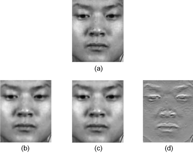
(b)Upper right... 28 Figure 2.10: Formation of HOOF with four bins... 30 Figure 2.11: Optical flow and optical strain computed between the onset and
apex frames. Visualization of (a) Horizontal optical flow; (b)
Figure 2.12: The eyes are masked for privacy concerns. Face is segmented into: (a) Three regions (i.e., forehead, cheeks, and mouth) (Shreve et al., 2009); (b) Eight regions (i.e., forehead, left and right of eye, left and right of cheek, left and right of mouth and chin) (Shreve, Godavarthy, et al., 2011); (c) Four regions (i.e., upper left, lower
left, upper right and lower right) (Shreve et al., 2014) ... 35 Figure 2.13: (a) SMIC sample images; (b) Video mapping on the curve by
adopting TIM to produce a new video ... 39 Figure 2.14: The acquisition setup for micro-expression elicitation of SMIC II
database ... 40 Figure 2.15: Example of short and long videos with onset, apex and offset
annotations... 41 Figure 2.16: The acquisition setup for micro-expression elicitation of CASME
II database... 50
Figure 3.1: Example of AUs of the FACS and their interpretations, adapted
from (Y. Zhang & Ji, 2005) ... 58 Figure 3.2: An example of a micro-expression video with onset-apex-offset
frame annotation, showing a ‘Surprise’ expression... 59 Figure 3.3: Examples of the emotion and AU labels (facial movements are
highlighted) in CASME II database (Yan, Li, et al., 2014) : (a) Fear - AU 20; (b) Sadness - AU 1; (c) Disgust - AU L4; (d)
Happiness - AU R12; (e) Surprise - AU R2 ... 61 Figure 3.4: Regions of interest suggested by: (a) Zhong et al. (Zhong et al.,
2015); (b) Happy and Routray(Happy & Routray, 2015); (c) Anderson and McOwan(Anderson & McOwan, 2006); (d) Wang et
al. (S. J. Wang, Yan, et al., 2014) ... 63 Figure 3.5: Example of annotating the 66 landmark coordinates using DRMF
method on a CASME II image ... 64 Figure 3.6: Flowchart of the proposed hybrid regions of interest extraction method . 68 Figure 3.7: Cropping out the three RoIs: (a) The 66 landmark points marked
by DRMF; (b) The rectangular boxes are set based on the
coordinate of the 12 landmark points of the four borders ... 71 Figure 3.8: Optical strain feature extraction for the first video after cropping
out the RoIs: (a) Original frames, f1,j; (b) Strain maps,m1,j; (c) Temporal pooled strain map; (d) Maximum-normalized and
resized frame ... 74 Figure 3.9: Comparison of the normalized optical strain magnitude between
the three RoIs (taken together) and the entire face region along a
Figure 3.10: Features of the first two blocks volumes extracted by using block-based LBP-TOP: (a) Each RoI is partitioned into 3×3 blocks; (b) LBP features generated fromXY,X T andY T planes; (c) Concatenation of features in each block into a single histogram;
(d) Concatenation of block histograms to form the final histogram... 77 Figure 3.11: A sample video sequence of ‘Surprise’ micro-expression from
SMIC-HS dataset... 79 Figure 3.12: Results (Percentage of improvement in accuracy over baseline) of
various combination of parameter settings by holding the value of: (a)win OSF,r∈[15,20]; (b)win LBP-TOP,N∈[3,4]; (c)rin
OSF,w∈[6,10], and; (d)Nin LBP-TOP,w∈[6,10]... 81 Figure 3.13: The percentage of improvement in recognition accuracy achieved
by varying parameterswwithrorN using: (a) OSF method for SMIC-HS; (b) LBP-TOP method for SMIC-HS; (c) OSF method
for CASME II; (d) LBP-TOP method for CASME II ... 86
Figure 4.1: Overview of the proposed algorithm ... 95 Figure 4.2: Effect ofτl andτuvalues on micro-expression recognition rate for
the SMIC-HS database ... 97 Figure 4.3: Example of vertical segmentation of the optical strain frame into
three regions ... 98 Figure 4.4: Extracting OSF from a sample video sequence: (a) Original
images, f1,j; (b) Optical strain mapsm1,j; (c) Images after
pre-processing; (d) Temporal pooled strain image; (e) Normalized
and resized strain image ... 99 Figure 4.5: OSW histogram formation: (a) Each j-th frame inm1,jis divided
into 5×5 blocks before the values ofεx,ywithin each block region are spatially pooled; (b) The block-wise strain magnitudeszb1,b2
from all frames(j∈1. . .Fi−1)are temporally mean pooled; (c) The weighting matrixWof sizeN×N is formed; (d) Coefficients
ofWare multiplied by their respectiveXY-plane histogram bins ... 101 Figure 4.6: Top row: a sample image from SMIC-HS (left) and the
corresponding optical strain map (right). Bottom row: a sample image from CASME II (left) and the corresponding optical strain
map (right). Noise block at the bottom left and right corners are marked 103 Figure 4.7: Micro-averaged accuracy results of the baseline (LBP-TOP) and
OSW methods using different LBP-TOP radii parameters on
SMIC-HS database based on LOSOCV ... 112 Figure 4.8: Recognition accuracy results of the baseline (LBP-TOP) and OSF
+ OSW methods using different block partitions in LBP-TOP. The
Figure 5.1: Flowchart of the apex frame spotting and emotion recognition system... 119 Figure 5.2: An example of a long and short video with annotated ground-truth
labels indicating the onset, apex and offset frames ... 121 Figure 5.3: Flow diagram of apex frame spotting in short video... 126 Figure 5.4: Demonstration of the apex frame spotting in a video sequence
using LBP feature extractor withdivide & conquerstrategy ... 130 Figure 5.5: Flow diagram of apex frame spotting in long video... 131 Figure 5.6: Eye masking process: (a) There are 6 landmark coordinates which
marked the boundaries of the left (landmark points 37, 38, 39, 40, 41 and 42) and 6 on the right (landmark points 43, 44, 45, 46, 47 and 48) eye regions; (b) The eye regions are removed after adding
some pixel margins... 132 Figure 5.7: Illustration of extraction of the three RoIs: (a) 66 landmark
coordinates labeled by DRMF; (b) The four edges (i.e., top, bottom, left and right) are determined based on the landmark point
locations; (c) Each RoI is partitioned into four blocks with the same size133 Figure 5.8: Obtaining Bi-Weighted Oriented Optical Flow (Bi-WOOF) features... 135 Figure 5.9: Bi-WOOF features formation: (a)θ andρ images are divided into
N×Nblocks. In each block, the values ofρfor each pixel are
treated as local weights to be multiplied with their respectiveθ
histogram bins; (b) It forms a locally weighted HOOF with feature size ofN×N×C; (c)ζb1,b2denotes the global weighting matrix,
which is derived fromεimage; (d) Finally,ζb1,b2are multiplied
with their corresponding locally weighted HOOF ... 138 Figure 5.10: Illustration of components derived from optical flow using the
apex and first frames of a video: (a) Horizontal vector of optical flow, p; (b) Vertical vector of optical flow,q; (c) Orientation,θ; (d)
Magnitude,ρ; (e) Optical strain,ε... 145
Figure 5.11: Top row without eye masking, bottom row with eye masking: (a-b) First frame in the video; (c-d) Spotted apex frame; (e-f)
Ground-truth apex frame; (g-h) Plots of optical strain magnitudes
LIST OF TABLES
Table 2.1: Recognition accuracy in CASME II using different combination of
radii values with fixed block size and neighboring points ... 27 Table 2.2: Detailed information of the SMIC database ... 38 Table 2.3: Detailed information of the SMIC-HS, SMIC-VIS and SMIC-HR
datasets ... 42 Table 2.4: Detailed information of the SMIC-E-HS, SMIC-E-VIS and
SMIC-E-NIR datasets ... 45 Table 2.5: Detailed information of CASME A and CASME B databases... 48 Table 2.6: Detailed information of the CASME II and CASME II-RAW databases.. 51 Table 2.7: General information of the USF-HD, Polikovsky’s and YorkDDT
databases ... 51
Table 3.1: Emotion description in terms of facial action units ... 69 Table 3.2: Frequency of the face regions based on the action units for five emotions 69 Table 3.3: The landmark points determining the corresponding RoIs bounding
boxes ... 70 Table 3.4: Reproduced baseline recognition results (%)... 84 Table 3.5: F-measure, recall and precision scores of the proposedRoI-selective
approach against their respective baselines in four different
scenarios (averaging across the good parameter ranges in Figure 3.13).... 88 Table 3.6: Comparison of recognition results of the proposed method to
existing methods in measurements of Accuracy, F-measure, recall
and precision scores in LOSOCV protocol... 89
Table 4.1: Micro-expression detection and recognition results on SMIC-HS
and CASME II database with LBP-TOP of 5×5 block partitioning ... 107 Table 4.2: Micro-expression detection and recognition results on SMIC-HS
and CASME II database with LBP-TOP of 8×8 block partitioning ... 107 Table 4.3: Confusion matrices of baseline and OSF + OSW methods for
detection task on SMIC-HS database with LBP-TOP of 5×5 block
partitioning ... 108 Table 4.4: Confusion matrices of baseline and OSF + OSW methods for
Table 4.5: Confusion matrices of baseline and OSF + OSW methods for recognition task on CASME II database with LBP-TOP of 5×5
block partitioning ... 109 Table 4.6: F-measure, recall and precision scores for detection and recognition
performance on SMIC-HS and CASME II database with LBP-TOP
of 5×5 block partitioning... 110 Table 4.7: F-measure, recall and precision scores for detection and recognition
performance on SMIC-HS and CASME II database with LBP-TOP
of 8×8 block partitioning... 111 Table 4.8: Comparison of micro-expression detection and recognition
accuracy results on the SMIC-HS and CASME II databases for
different feature extraction methods ... 115
Table 5.1: Comparison of micro-expression recognition performance in terms of F-measure on the CASME II, SMIC-HS, SMIC-VIS and
SMIC-NIR databases for the state-of-the-art feature extraction
methods, random frame selection approach, and the proposed algorithm. 142 Table 5.2: Confusion matrices of baseline and Bi-WOOF (apex & first frame)
for recognition task on the CASME II database ... 143 Table 5.3: Confusion matrices of baseline and Bi-WOOF (apex & first frame)
for recognition task on the SMIC-HS database ... 144 Table 5.4: Performance of apex frame spotting with and without eye masking
on the CASME II-RAW database measured by MAE. ... 148 Table 5.5: Performance of apex frame spotting with and without eye masking
on the long videos databases measured by ASR... 148 Table 5.6: Recognition performance for long videos in terms of F-measure ... 149 Table 5.7: Comparison of the recognition accuracy between the state-of-the-art
method and the proposed method on the SMIC-E-VIS database ... 149 Table 5.8: Average number of frames in the short and long videos of the
CASME II and three SMIC databases ... 152 Table 5.9: Confusion matrices for the recognition task on the
LIST OF SYMBOLS AND ABBREVIATIONS
Fi : Total number of frames in a video.
M : LBP-TOP Histogram.
N×N : Block partitioning.
P : Number of neighbor points.
R : Radii.
X : Width of an image.
Y : Height of an image.
M : Normalized LBP-TOP Histogram.
ε : Optical strain magnitude.
~u : Displacement vector.
fi,j : Frame indices.
mi,j : Strain map.
n : Total number of video sequence in the database.
p : Horizontal component of optical flow vector.
q : Vertical component of optical flow vector.
si : Number of video in the database.
AAM : Active Appearance Model.
ASM : Active Shape Model.
ASR : Apex Spotting Rate.
AU : Action Unit.
Bi-WOOF : Bi-Weighted Oriented Optical Flow.
CASME II : Chinese Academy of Sciences
Micro-Expression II.
CK+ : Extended Cohn Kanade.
CLM : Constrained Local Model.
DRMF : Discriminative Response Map Fitting.
DTSA : Discriminant Tensor Subspace Analysis.
ELM : Extreme Learning Machine.
ERI : Expression Ratio Image.
FACS : Facial Action Coding System.
FERET : Facial Recognition Technology.
HOG : Histogram of Gradient.
HOOF : Histogram of Oriented Optical Flow.
LBP : Local Binary Pattern.
LBP-SIP : Local Binary Patterns with Six Intersection Points.
LBP-TOP : Local Binary Pattern on Three Orthogonal
Planes.
LOVOCV : Leave-One-Video-Out Cross Validation. LSTD : Local Spatio-temporal Directional Features.
LWM : Local Weighted Mean.
MAE : Mean Absolute Error.
MKL : Multiple Kernel Learning.
OF : Optical Flow.
ORL : Olivetti Research Laboratory.
OS : Optical Strain.
OSF + OSW : Concatenation the OSF and OSW.
OSW : Optical Strain Weighted Features.
RF : Random Forest.
riLBP : Rotation Invariant LBP.
riuLBP : Uniform Rotation Invariant LBP.
RoI : Region of Interest.
SMIC : Spontaneous Micro-expression.
SVM : Support Vector Machine.
TIM : Temporal Interpolation Model.
LIST OF APPENDICES
CHAPTER 1: INTRODUCTION
1.1 Understanding Micro-expression
Facial expression is the most common form of non-verbal communication that displays a person’s feeling. It is also known as the universal language of emotion as it is shared among different cultures. There are six basic classes of emotions, notably happiness, sur-prise, anger, sad, fear and disgust (Ekman & Friesen, 1971). In general, facial expression can be categorized into two main types: macro-expression and micro-expression. Macro-expression, also known as the normal Macro-expression, is usually obvious and can be easily identified in real-time with the naked eye. However, since macro-expression is a volun-tary expression, it can be exploited to deceive others by imitating or acting out the falsified expressions and portray them on the face. More precisely, macro-expression goes on and off on the face, normally between three quarters of a second to two seconds (Shreve et al., 2009), and can be found at multiple large areas of the face. Automatic macro-expression recognition is a popular research field and has been intensively studied over the past two decades.
On the other hand, in recent years, analysis of micro-expression has also attracted more and more attention in the field of computer vision. Yet, not many papers have been published. This is because micro-expression has shorter duration (micro) and lower intensity (subtle) (Ekman & Friesen, 1969). It often occurs at high speed and usually sustains within one-fifth to one-twenty-fifth of a second (Porter & Ten Brinke, 2008). Due to its extremely brief and rapid facial muscle movement, as well as the fact that it may only appear in a few small parts of the face, it is technically challenging to realize and recognize the micro-expressions in real-time conversations, except for the keen and trained observers (Ekman, 2009b).
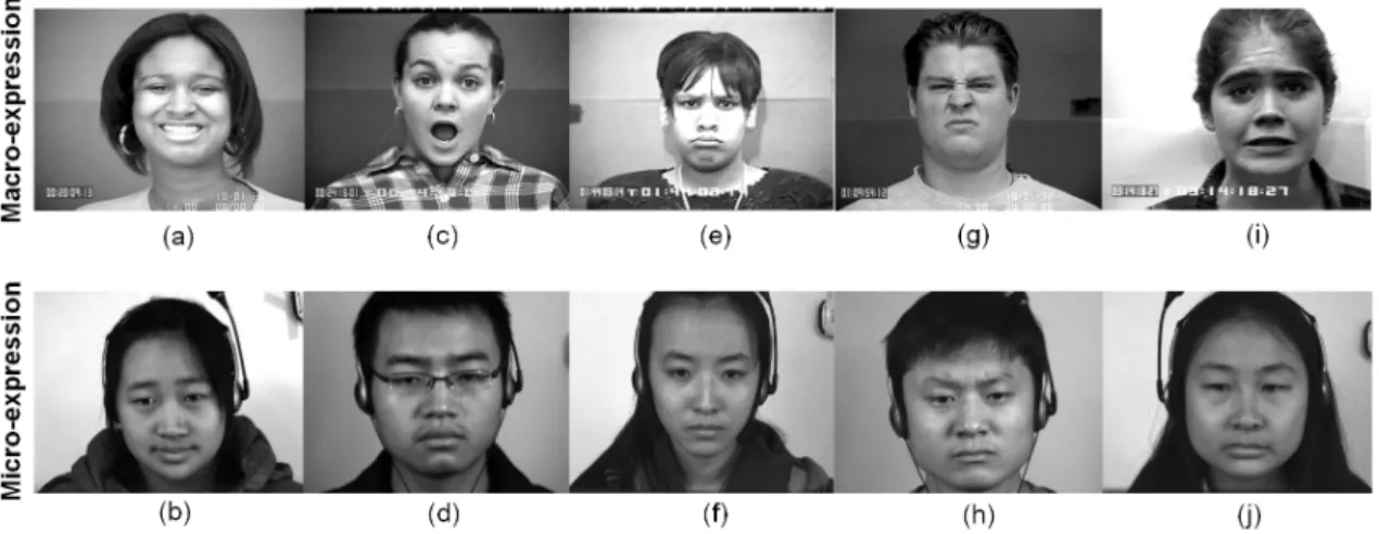
Figure 1.1: The top row of images show some examples of macro-expression (from CK+ database) and the second row of images show examples of micro-expression (from CASME II database). The emotion types are: (a-b) happiness, (c-d) surprise, (e-f) sad-ness, (g-h) disgust and (i-j): fear
Micro-expressions are provoked involuntary and spontaneously. In other words, it is uncontrollable, and thus being able to reveal a person’s concealed genuine feel-ings (Ekman & Friesen, 1969). Figure 1.1 illustrates some images containing either the macro- and micro-expressions. The attributes between macro- and micro-expressions can clearly be differentiated using the figure shown. Specifically, the characteristics of micro-expression makes it advantageous to be recognized and studied, as we are able to interpret whether someone is concealing his feeling or is trying to tell a lie (Ekman, 2009a). For instance, the suspects interrogated by the police can be caught lying. Analyzing a per-son’s emotion can also help improve relationships and understand each other better. In addition, we can become more aware of our own emotions and manage them more effec-tively. In short, recognition of micro-expressions is beneficial in both our mundane lives and also society at large. It can be utilized in a wide range of applications, such as med-ical diagnosis, community safety, business negotiation, social interactions, etc. (Frank, Herbasz, et al., 2009; O’Sullivan et al., 2009; Frank, Maccario, & Govindaraju, 2009).
Micro-expressions have been studied intensively in the field of psychology. The first discovery of micro-expression was made by Haggard and Isaacs (Haggard & Isaacs, 1966), who named it as “micromomentary expression (MME)” and considered it as
re-pressed emotion. They stumbled upon it while performing analysis on a psychotherapeu-tic interview film, where they viewed the film frame-by-frame to understand the patient’s thinking. They observed that the emotion shown by the patient changed dramatically within three to five frames. Few years later, Ekman and Friesen (Ekman & Friesen, 1969) introduced the termmicro-expressionfrom a case where the patient was trying to conceal his sad feeling by concealing it with a smile. The therapist detected his genuine feeling by carefully observing the subtle movements on his face. In fact, the patient was planning to commit suicide. In addition, they discovered that people who are trying to deceive others are more likely to attempt in disguising their facial behavior than body movements (Ekman & Friesen, 1974).
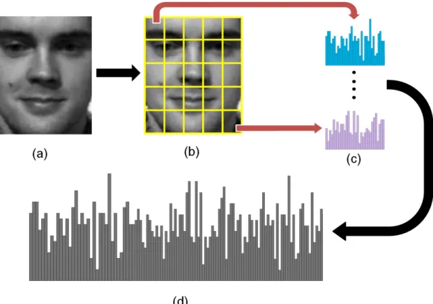
1.2 General framework of a Micro-expression Recognition System
There are three main components in a general facial micro-expression recognition sys-tem, as illustrated in Figure 1.2. The input of the recognition system is the raw images, which are extracted from video sequences. The first stage of the system is pre-processing, which aims to enhance the image features for further analysis. Pre-processing includes smoothening the distorted image caused by illumination and lighting effects, normalizing the pixel intensity or scaling the brightness level distribution of the image affected by non-uniform light, face registration and alignment to transform and standardize all faces into a uniform size and shape based on a template face, etc. Next, the feature extraction process combines the large set of raw image data into a compact and discriminative fea-ture vector. This process forms a compact representation of the image data by reducing the feature dimension. The resultant feature vector is able to describe the color, shape, texture and motion which exist in the image. It is also robust to translation, noise, oc-clusion, rotation, illuminations and scaling. The last step of the system is classification, which categorizes the emotion classes of the testing data based on the defined training
Figure 1.2: Block diagram of a facial micro-expression recognition system
data. It involves a learning algorithm that analyzes and organizes the training data into a finite desired group of clusters with respect to the emotion classes. Then, the emotion type of the testing data is determined based on the distance or similarity measure. This thesis focuses on the first two stages, namely pre-processing and feature extraction. In this research, several efficient and improved pre-processing and feature extraction tech-niques are proposed and implemented. Results show that they are capable of producing better recognition performances compared to the current state-of-the-art techniques.
1.3 Problem Statements
As previously explained, the study of micro-expression is still considered as a relatively new topic compared to that of macro-expression. For macro-expression, there are nu-merous well-established databases that are publicly available for benchmarking and eval-uation purpose. Hence, many macro-expression recognition mechanisms have been de-signed to detect and classify a person’s emotional state. Some of them are robust to operate in the wild (or the real world environment) and real-time scenario, while others manage to achieve perfect classification accuracies (around 100%) in certain databases.
On the contrary, the subtlety and minuteness of micro-expressions have profoundly hindered the progress of its related research works. To date, there are only a few micro-expression databases with proper data elicitation which provide complete ground-truths, due to the challenges of triggering the involuntary spontaneous expressions. This brings to an even greater obstacle in the development of micro-expression detection and recog-nition algorithms. In the literature, most state-of-the-art techniques achieve poor
recogni-videos which do not consist of micro-expression-unrelated motion. Furthermore, the pre-processing and feature extraction techniques employed in these systems are initially meant for macro-expression analysis, and may not perform well for micro-expressions due to different attributes and characteristics.
Until now, the labeling of ground-truths for micro-expressions are still performed manually by trained psychologists or professional experts. The drawbacks of the hand-labeled practice include: (a) inconsistent reliability - the labels may differ from person to person; (b) time consuming - requires great amount of effort and concentration for frame-by-frame evaluation; (c) costly - requires specific trained experts. The aforementioned issues indicate that it is essential to label the ground-truths automatically. Although there are some automatic micro-expression detection and recognition systems, there are still rooms for improvement. In summary, the problem statements for this research are as follows:
1. Poor performances by existing micro-expression detection and recognition systems due to the challenges in capturing the quick and minute micro-expressions.
2. Limited scope of exploration in pre-processing stage for micro-expression analysis.
3. Similar facial motion patterns appearing in consecutive frames implies redundancy and leads to a less discriminative set of features.
1.4 Objectives
This thesis aims to improve the current micro-expression detection and recognition sys-tems by studying the pre-processing and feature extraction approaches. The primary ob-jectives of this research are set out as follows:
1. To design a spatio-temporal feature extractor that can effectively describe the local appearance of micro-expressions.
2. To develop a pre-processing method that removes unwanted facial areas for con-centrating only on regions that contribute meaningful micro-expression details.
3. To demonstrate that it is sufficient to consider only one frame out of the whole video sequence when extracting facial micro-expression features for recognition task.
1.5 Scopes and Limitations
The scope and limitation of this study are as follows:
1. The types of emotion for micro-expression classification are strictly limited to only the emotions provided in the databases. No other types of emotion or subjects’ feeling (i.e., anxiety, guilty, relief, etc.) are analyzed.
2. The databases used in the experiments are elicited under constrained laboratory conditions, which means that all the images have been pre-processed with face registration and alignment. There is no micro-expression database recorded in the wild.
3. The proposed pre-processing and feature extraction techniques are only tested on micro-expression videos.
4. To recognize the emotion type, only the muscle or skin tissue movements on the face are studied. Other features that may provide clues for micro-expressions, such as eye gaze and speech signals, are not considered.
1.6 Contributions
Most existing pre-processing and feature extraction approaches applied on the micro ex-pression videos are designed for macro-exex-pression analysis. In this thesis, the weaknesses of these approaches are addressed and solutions are provided to mitigate the issues. The
RoI-Selective: A hybrid facial region selection technique, RoI-Selectiveis proposed to
extract several important parts of the face that contain significant and valuable micro-expression information. More precisely, it combines heuristic-based and automatic ap-proaches to exclusively determine the salient facial regions. The heuristic-based approach relies statistically on the occurrence frequency of the facial action units for all the expres-sions, whereas the automatic detection of the landmark points is performed using a robust landmark detector. This work has been submitted to the Journal of Signal Processing Systems (JSPS).
OSW + OSF:For micro-expression detection and recognition, three distinct spatio-temporal
feature extraction techniques are developed by utilizing optical strain magnitude. Optical strain is the extension of optical flow that has a higher order derivative, and possesses the ability to eliminate noises and preserve relative large facial muscle changes. For the three feature extraction techniques: (a) OSW- the optical strain magnitude is formulated as a weighting scheme to scale the values of the feature obtained by a baseline feature extrac-tor called LBP-TOP; (b) OSF - the temporal details for each frame, which are derived from optical strain technique, are summed up to create a compact and efficient feature vector, and; (c) OSW + OSF - the two sets of features (i.e., OSWand OSF) are com-bined to form a more representative feature histogram. This work has been published in the Asian Conference on Computer Vision Workshops (ACCVW 2014), Intelligent Signal Processing and Communication Systems (ISPACS 2014) and Signal Processing: Image Communication (SPIC).
Single Apex: Apex frame in a micro expression video sequence is the frame that depicts
the most expressive emotional state. Apex frame lies between the onset and offset frames, which are the instant of the beginning and ending of the micro-expression, respectively.
In this research, a single apex frame is utilized to represent the entire video. An auto-matic apex frame spotting approach is established to allocate the apex frame for various scenarios, including short and long videos, with and without onset and offset frame in-formation. Moreover, a novel feature descriptor calledBi-WOOFis developed to encode the features obtained from the spotted apex frame. This work has been published in the IAPR Asian Conference on Pattern Recognition (ACPR2015). The extended work has been submitted to the Asian Conference on Computer Vision Workshop (ACCVW 2016) and Neurocomputing Journal.
1.7 Structure of Thesis
This thesis is organized into six chapters. The contents for each chapter, except for Chap-ter 1, are outlined briefly in this section. ChapChap-ter 2 provides liChap-terature review on exist-ing image pre-processexist-ing and feature extraction algorithms, as well as micro-expression databases. In addition, the pros and cons for each method and database are discussed. In Chapter 3, a novel pre-processing method is proposed, which emphasizes on impor-tant facial regions to boost the micro-expression recognition performance. Chapter 4 describes the three distinct feature extractors, which have been devised from the optical strain technique. They are capable of encoding the subtle and short elapsed occurrence of micro-expressions. Apart from the conventional feature extractors that consider the entire video sequence or a sub-sequence of it for representation, Chapter 5 proposes a new ap-proach, which expresses the features of a video based on only a single frame. Chapter 6 draws some conclusions and suggests possible future research directions.
CHAPTER 2: LITERATURE REVIEW
2.1 Overview
The materials in the literature are studied and presented in this chapter. Firstly, the tech-niques used in pre-processing are reviewed. Next, some of the popular feature extractors are discussed. Then, all the publicly available micro-expression databases are reviewed. Finally, the problems faced by the surveyed literature are identified and discussed.
2.2 Overview of Image Pre-processing
As discussed in Chapter 1.2, it is essential to pre-process the raw micro-expression videos before conducting any experiment on the datasets. There are several pre-processing tech-niques in the literature which can effectively extract the image features resulting in better performances. Three widely-used pre-processing methods are studied, namely: (a) face registration and alignment; (b) image filtering, and; (c) facial region extraction. Each pre-processing methodology mentioned are detailed in the following sub-chapters.
2.2.1 Face Registration and Alignment
Due to the spontaneity of micro-expressions, the databases (i.e., Spontaneous Micro-expression (SMIC) (Pfister et al., 2011) and Chinese Academy of Sciences Micro-Expression II (CASME II) (Yan, Li, et al., 2014)) have gone through face registration and alignment processes before being released to the public. Although the datasets are collected under constrained laboratory condition, the external factors that contribute to feature noises, such as head movement and the shape of the face, need to be properly addressed.
There are four main steps involved in this process, namely:
1. Model face selection - a frontal face image with neutral expression is detected and selected as the model face (i.e., as the reference).
2. Landmark coordinate detection - a detector to allocate the facial landmark coordi-nates is adopted. Note that the terms facial landmark coordinate and facial fea-ture pointare used interchangeably in this thesis and will be selected based on the suitability of the context. Typically, there are three techniques commonly used in locating the facial feature points, namely:Active Shape Model (ASM) (Van Gin-neken et al., 2002), Constrained Local Model (CLM) (Cristinacce & Cootes, 2006) and Active Appearance Model (AAM) (Cootes et al., 1998). ASM is employed to detect the facial landmark points in the micro-expression databases (i.e., SMIC and CASME II). It is a statistical model of the shape of an object that are repeti-tively deformed to fit a sample object. ASM is capable of spotting a total of sixty eight landmark coordinates on the face. The search commences from a mean shape aligned to the position and size of the face determined by a face detector. Then, the processes are iterated until convergence.
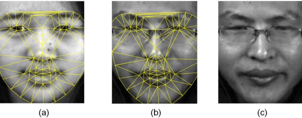
3. Face transformation - the first frame of each micro-expression sequence is normal-ized to the model face using a Local Weighted Mean (LWM) (Goshtasby, 1988) transformation. The rest of the frames are transformed and normalized using the same transformation matrix. The reason of using the same transformation matrix is that the occurrence of the micro-expression is too rapid, and the rigid head move-ment within the duration can be ignored. Additionally, the ASM landmark detector may not be sufficiently accurate thus it could cause a significant deviation of loca-tions for the same points even when the face remains stationary. Figure 2.1 shows an example of face transformation.
4. Face normalization - the eye coordinates of the first frame for each normalized micro-expressions video clip are located and the face of each frame is cropped based on the rectangle determined by the eye coordinates.
Figure 2.1: Face transformation. (a) Model face with feature points detected; (b) Sample face before transformation; (c) Results of mapping the feature points from sample face to model face
2.2.2 Image Filtering
In addition to the noise introduced by the capturing device and environment, other factors including clothing and headset wire may affect the performance of a micro-expression recognition system. Since the motions characterized by the subtle facial expressions are very fine, it is likely that the presence of the unwarranted noises will generate false infor-mation to the micro-expression recognition system. Thus, a feasible pre-processing tech-nique is required to suppress the unwanted noise to better describe the micro-expressions. Image filtering is a simple mathematical processing tool that is accomplished through a convolution operation. It is also a standard process that applies to almost all the im-age processing systems. Among the filtering processes, smoothing and blurring are the common ones, with adjustable levels to accommodate for different conditions and appli-cations. Various types of filter are proposed in the literature, including Gaussian, Wiener, Sobel, Canny, Prewitt and Roberts. Three prominent image filters are chosen and dis-cussed in this section, namely, Gaussian, Wiener and Sobel filters.
Gaussian filter is an adaptive filter controlled by a set of parameters based on an optimization algorithm (Forsyth & Ponce, 2002). It is a low pass filter as it removes high-frequency components from the image. The Gaussian filter formula can be expressed as
follows: G(x,y) = 1 2π σ2 e− x2+y2 2σ2 , (2.1)
whereσ is the standard deviation of the Gaussian distribution. It is effective for
remov-ing Gaussian noises from image. In the work by Liu et al. (Z. Liu et al., 2001), Gaussian filter is adopted to minimize the noises on image in order to compute the change of il-lumination of a person or Expression Ratio Image (ERI) resulting from deformation of the person’s face. The main reason Gaussian filter is chosen is that the degree of smooth-ing on the face can be tailored, where little smoothsmooth-ing is applied on expressional areas, while significant smoothing in the remaining areas. In other words, different treatment is applied to different region. Besides that, Gaussian filter is applied as the fundamental step for the cross-modality 2D-3D face recognition analysis (Jin et al., 2014). It is the pre-processing step for data enhancement by removing the noise spikes (i.e., the pixels that have exceptionally low or high pixel intensity values) on the face image collected. Despite the wide application of Gaussian filter, its smoothing process may reduce the fine image details. In this study of micro-expression recognition system, the subtle changes are particularly important. Thus, adjusting the Gaussian window to an optimal value is es-sential to efficiently filter out the noises while keeping the meaningful information about fine expression.
On the other hand, Wiener filter is a classic filter that is based on linear time-invariant estimation of an image (Goldstein et al., 1998). It is a low pass filter that finds the best reconstruction of a noisy signal by suppressing the overall mean square error in the inverse filtering and noise smoothing stages. It is able to remove noises that corrupt the signals. Wiener filter is often applied in the frequency domain. The image after taking the product
of the Wiener filterW(u,v)is estimated as follows:
ˆ
G(u,v) =W(u,v)O(u,v), (2.2)
where O(u,v) is the Discrete Fourier Transform of the original image O(x,y). In the application of digital image binarization to preserve useful texture information for low quality digitized documents, Wiener filter has demonstrated its efficiency in removing the noise areas by highlighting the contrast between background noise and text areas, while maintaining the desired image features (Gatos et al., 2004). In addition, Wiener filter has extended its efficacy to patch-based Wiener filter that can achieve near-optimal denoising (Chatterjee & Milanfar, 2012). It uses both the geometrically and photometrically similar patches to accurately estimate and learn the parameters. The denoising approach achieved promising performance on both grayscale and color images. It is worth noting that the parameters of the method are obtained from analytical formulation and they do not require further fine-tuning.
Last but not least, Sobel filter, also known as the Sobel-Feldman operator, has been widely used long before the inception of Gaussian filter and its derivatives. It is a pair of 3
×3 convolution masks that estimates the gradients of pixel intensity in the horizontal and vertical directions. Each pixel in the image is convolved by differentiating two rows or two columns to calculate the gradient. The Sobel gradient approximation for each pixel in an image is expressed as:
|G|= q
Gx2+Gy2, (2.3)
whereGx andGyare the approximated derivatives of the pixels in the horizontal and ver-tical directions. The main advantage of Sobel filter is its high sensitivity towards noises, enabling it to highlight the important edges in an image. Pai et al. (Pai & Chang, 2011)
applied Sobel operator to produce a binary edge image (i.e., 1 indicates edge pixel and 0 denotes no edge) that has clear contrast between the face contour and background. The face and the background are successfully outlined accurately using the skin tone-segmenting processes. Furthermore, the dominant facial features such as the mouth and eyes regions are highlighted precisely, hence improving the subsequent recognition task. Another example of the application of Sobel filter is in skin color detection (Lamsal & Matsumoto, 2015). The skin color detector is modified by combining it with the Sobel edge detector (Viola & Jones, 2004). This method produces promising face detection per-formance, and is able to detect both the color and grayscale images in three facial image databases. However, Sobel filter is susceptible to noise. As the noise level increases, the magnitude of the edges decreases, thus affecting the edge detection accuracy.
Figure 2.2 illustrates the output of pre-processing the same image with three different filters (i.e., Gaussian, Wiener and Sobel filter) discussed above.
2.2.3 Facial Region Selection
Many research papers demonstrated that extracting features from partial face is able to achieve better facial expression recognition performance, compared to when considering the entire face (Shan & Gritti, 2008; Fan & Verma, 2009). The main reason is that, these local facial patches contribute more expressional information towards distinguishing the expressions, and at the same time, eliminating the parts that do not correspond to the desired facial movements.
Shan and Gritti (Shan & Gritti, 2008) elicited a finite set of discriminative Regions of Interest (RoIs) that is more representative, instead of considering the entire face image. For their methodology, the face image is first divided into several sub-regions, before us-ing the Local Binary Pattern (LBP) (Ojala et al., 1996) feature descriptor to capture the local appearance in region level. Finally, the weak classifer Adaboost (Schapire & Singer,
Figure 2.2: A face image before and after applying the filters. (a) Original image; (b) Gaussian filter; (c) Wiener filter; (d) Sobel filter
1999) is employed to learn and identify the most discriminative sub-regions (in term of LBP histogram). The method is tested on a facial expression database (i.e., Extended Cohn Kanade (CK+) (Lucey et al., 2010)), and attains consistently good recognition per-formances when three different classifiers are adopted. The paper summarized that the important features are mostly attributed to the eyes and mouth regions. Figure 2.3 shows the top 20 discriminative sub-regions selected for each individual expression. Nonethe-less, the selection of the feature length is determined statistically based on the plot of recognition rate against the number of features.
Fan and Verma (Fan & Verma, 2009) discovered a combination of RoIs that contain the most important subtle facial motion information. These RoIs are “left eye region”, “right eye region”, “nose region” and “mouth region”. For analysis, the facial expression recognition performances are reported separately for each facial region. They discover
Figure 2.3: Sub-regions selected for the facial expressions: (a) Anger; (b) Disgust; (c) Fear; (d) Joy; (e) Sadness; (f) Surprise; (g) Neutral
that eyes and mouth achieve better recognition performance than the other facial regions, such as nose. By locating the most significant areas on the face, an excellent classification accuracy of 94% is obtained on the face benchmark database, i.e., Facial Recognition Technology (FERET) (Phillips et al., 1998). However, the size of the facial patches is sensitive to the feature representation and is completely based on empirically determined findings from numerous experiments.
2.3 Overview of Feature Extraction
Feature extraction process plays a vital role in a wide range of computer vision tasks, such as object recognition, image restoration, scene reconstruction, etc. Its main function is to reduce the image attributes from high dimensional feature space to a lower dimension. The resultant features possess more meaningful and richer information to better represent the original image, thereby facilitating the analysis of interest. In this sub-chapter, four popular low level feature descriptors, which are considered in this study, are described
in detail, namely: (a) LBP; (b) Local Binary Pattern on Three Orthogonal Planes (LBP-TOP); (c) Optical Flow (OF), and; (d) Optical Strain (OS). A low level feature refers to the component which directly deals with pixel intensities, for instance, color, texture, shape, edge and corner.
2.3.1 Local Binary Pattern
LBP feature descriptor, which was first introduced by Ojala et al. in 1996 (Ojala et al., 1996), is originally designed for texture analysis. It is an effective image feature descriptor, not only used for texture interpretation, but has also been further extended to various fields in computer vision due to its advantage of: (a) discrimination ability; (b) compact texture representation; (c) low computational complexity, as well as; (d) invariant to any monotonic gray-level changes. Examples of its application include face recognition (Xi et al., 2016), facial expression classification (Zhao & Pietikainen, 2007), event detection (Ma & Cisar, 2009) and even medical image analysis (Nanni et al., 2010; Mirmohamadsadeghi & Drygajlo, 2011).
LBP operator is a robust descriptor that represents a two-dimensional gray-scale im-age by converting pixel values into binarized pattern. The concept of LBP operator is simple, where the intensity value of the center pixel is compared to its circular neighbor-ing pixels usneighbor-ing a thresholdneighbor-ing technique. Specifically, given a pixelcat position(xc,yc), the binary code is computed by comparing the value of pixelcwith its neighboring pixels:
LBPP,R(xc,yc) = P−1
∑
p=0 s(gp−gc)2P,s(x) = 1, x≥0; 0, x<0, (2.4)wherePdenotes the number of neighboring points equally sampled on a circle of radius
R. gc is the gray value of the center pixel and gp is the gray value of the pixels equally sampled points around the circular neighborhood of radius R, and 2P is the weight
cor-Figure 2.4: Example of three different circularly symmetric neighbor sets, [P,R]: (a) [4,1]; (b) [8,1]; (c) [8,2]
responding to the neighboring pixels. Figure 2.4 shows different [P,R] sets of circular neighborhood. Figure 2.5 illustrates the basic LBP operator , where each pixel in the 3×3 circular neighborhood is compared to pixel c. The 2P bins histogram is formed by calculating the occurrences of the LBP code derived across the whole face image.
Figur e 2.5: Illustration of processes in the basic LBP operator
LBP also provides different options for texture representation to reduce the number of histogram bins, such as Uniform LBP (uLBP), Rotation Invariant LBP (riLBP) and
Uniform Rotation Invariant LBP (riuLBP) (Ojala et al., 2002). Specifically, uLBP is a uniformity measure of pattern: if the total number of transitions from 0 to 1 or from 1 to 0 in the binary codes are less than or equal to 2, they are categorized as important. Otherwise, they are grouped into the miscellaneous bin in the histogram. For example, the patterns 000000002 (0 transition), 100000002 (1 transition) and 011000002 (2
tran-sitions) are uniform whereas the patterns 100010012 (4 transitions) and 110100102 (5
transitions) are not. For riLBP, it is achieved using rotation invariant mapping, where the binary code circularly rotates until reaching the minimum value. For instance, the patterns 0101100002 (17610), 0001011002 (4410) and 000010112 (1110) are all mapped
to the minimum code 000010112(1110).
The block-based LBP was introduced in 2004. It equally divides the face area into small regions (Ahonen et al., 2004). This is to ensure that the spatial appearance can be described locally on a regional level. Then, the regional features are concatenated to form a global description of the face. Figure 2.6 shows the steps of constructing the block-based LBP feature histogram. The effectiveness of this approach has been validated on two face databases (i.e., FERET (Phillips et al., 1998) and Olivetti Research Laboratory (ORL) (Samaria & Harter, 1994)). When comparing to other approaches developed for face recognition, block-based LBP shows its superiority and robustness against different facial expressions, lighting condition and aging of the subjects.
Nanni et al. (Nanni et al., 2010) presented several LBP variants by designing new en-coding schemes for the validation of the local gray-scale differences. Instead of adopting the original circular shape when thresholding the center pixel to the surrounding pix-els, four other neighborhood shapes are created, including, ellipse, parabola, hyperbola
Figure 2.6: Block-based LBP: (a) Face image; (b) Face equally divided into 5×5 blocks; (c) Histogram for each block; (d) Resultant feature histogram
Their methods are tested on three medical databases: (a) Infant COPE database (Brahnam et al., 2007) - to categorize the pain states from neonatal images; (b) 2D-HeLa database (Chebira et al., 2007) - to classify the protein localization starting from fluorescence mi-croscope images, and; (c) Pap smear database (Jantzen et al., 2005) - to detect abnormal smear cells. The elliptic neighborhood generates a reliable set of features in all three databases. Particularly in 2d-HeLa database, it outperformed all the texture descriptors in the literature.
The first work that applies LBP methodology on human detection task is demon-strated by Mu et al. (Mu et al., 2008). However, the ordinary LBP operator does not perform well in detecting the human in a personal album (i.e., INRIA human database (Dalal & Triggs, 2005)) due to high complexity and semantic consistency issues. Two feature descriptors, namely, Semantic-LBP and Fourier-LBP, are developed to address these problems. They are able to encode the features using a more compact
representa-Figure 2.7: Neighborhood topology of LBP for bio-imaging application: (a) Circular; (b) Ellipse; (c) Parabola; (d) Hyperbola; (e) Archimedean spiral
tion. Extensive experiments have been carried out to compare the methods with gradient-based feature descriptors. The better detection accuracy and higher computational speed achieved further confirm the feasibility of the binary codes in capturing meaningful local structures on image manifold.
2.3.2 Local Binary Pattern on Three Orthogonal Planes
In 2007, Zhao and Pietikainen (Zhao & Pietikainen, 2007) proposed an extension of the spatial LBP to spatio-temporal volumes, namely LBP-TOP. The original LBP descrip-tor describes two dimensional local spatial structure of an image, whereas LBP-TOP can describe the three dimensional dynamic textures of a video sequence. Rather than extracting the 2D (i.e., fromXY plane) features, the 3D variant of LBP considers the co-occurrence statistic on three orthogonal planes (i.e.,XY, XT andYT). The authors (Zhao & Pietikainen, 2007) listed several main advantages of LBP-TOP, namely: (a) capable of extracting the appearance and motion features in three directions; (b) ability to capture the local spatio-temporal transition information (i.e., pixel, region and volume levels); (c)
robustness to rotation, translation, illumination or skin color variation, gray-scale changes and even error in face alignment, as well as; (d) computational simplicity.
Similar to LBP, it has been extended to block-based LBP-TOP to describe more local attributes. Figure 2.8 shows the process of extracting the block-based LBP features from three orthogonal planes, followed by concatenating the computed local features into a resultant histogram.
e 2.8: Block-based LBP-T OP features extraction of the first tw o block v olumes from a video sequence: (a) Block v olumes; (b) LBP features three orthogonal planes; (c) Histogram concatenation of each block v olume from XY , XT and YT planes to form a single histogram; (d) Histogram from the tw o block v olumes
The concatenated histogram describes the global motion of the face over a video sequence, and it can be succinctly denoted asM:
Mb1,b2,d,c=
∑
x,y,tI{hd(x,y,t) =c} (2.5)
where c∈ {0, . . . ,2P−1}, d ∈ {0,1,2}, b1,b2 ∈ {1, . . . ,N}, and 2P is the number of
different labels produced by the LBP operator on thed-th plane for cased=0 refers to theXY plane, which describes the appearance; cased=1 refers to theX T plane, which describes the horizontal motion, and; cased=2 refers to theY T plane, which describes the vertical motion. As the LBP code cannot be computed at the borders of the 3D video volume, only the central part is taken into consideration. hd(x,y,t)is the LBP code, i.e., Equation (2.4), of the central pixel (x,y,t)on the d-th plane, for x∈ {0, . . . ,X−1},y∈ {0, . . . ,Y−1},andt∈ {0, . . . ,T−1}. X andY are the width and height of image (thus,
b1 and b2 are the row and column indices, respectively), while T is the video length. As such, the functional term I{A}determines the count of the c-th histogram bin when
hd(x,y,t) =c: I{A}= 1, ifAis true; 0, otherwise. (2.6)
Hence, the final feature histogram is of dimension 2P×3N2. For an appropriate compar-ison of the features among video samples of different spatial and temporal lengths, the concatenated histogram is sum-normalized to obtain a coherent descriptorM:
Mb1,b2,d,c= Mb1,b2,d,c nd−1 ∑ k=0 Mb1,b2,d,k . (2.7)
In this thesis, the LBP-TOP parameters are denoted by LBP-TOPPXY,PX T,PY T,RX,RY,RT where theP parameters indicate the number of neighbor points for each of the three or-thogonal planes, while theRparameters denote the radii along theX,Y, andT dimensions of the descriptor.
Unlike other feature extractors, LBP-TOP extracts the dynamic textures over space-time dimensions. Hence, it remains a popular choice of feature extraction method for var-ious applications, including gait and action recognition (Kellokumpu et al., 2009; Mattivi & Shao, 2009), face spoofing (Chingovska et al., 2013), depression analysis (Joshi et al., 2012) and facial expression recognition (Zhao & Pietikäinen, 2009).
Furthermore, LBP-TOP has became a baseline feature extractor in micro-expression analysis due to its high discriminating power and impressive texture representation, for instance, in the databases: (a) SMIC (Pfister et al., 2011); (b) SMIC II (Li et al., 2013); (c) CASME (Yan et al., 2013); (d) CASME II (Yan, Li, et al., 2014). Specifically, LBP-TOP is utilized to perform detection and recognition tasks, where the former aims to classify micro-expressions versus non-micro-expressions, while the latter is to classify the emotions into different categories (i.e., happiness, surprise, disgust, sadness and others). Different combination of the parameters (i.e., block size, radii and number of neighboring points) in LBP-TOP setting generates different detection and classification performance. Yan et al. (Yan, Li, et al., 2014) provides the recognition performances of different radii values (i.e., RX, RY andRT) with fixed 5×5 block size and neighboring points of 4 in CASME II database, as tabulated in Table 2.1. Among all the values tested, the best performance obtained is 63.41% when the radii areRX = 1,RY = 1 andRT = 4.
Wang et al. (Y. Wang et al., 2014) extended the LBP-TOP feature descriptor by proposing the Local Binary Patterns with Six Intersection Points (LBP-SIP), before eval-uating it in two micro-expression databases. LBP-SIP reduces redundant intersection
Table 2.1: Recognition accuracy in CASME II using different combination of radii values with fixed block size and neighboring points
RX RY RT Recognition Accuracy (%) 1 1 2 63.01 1 1 3 62.60 1 1 4 63.41 2 2 2 61.38 2 2 3 61.79 2 2 4 62.20 3 3 2 58.54 3 3 3 61.79 3 3 4 58.55 4 4 2 58.94 4 4 3 61.38 4 4 4 60.57
tation and lower computational complexity. With a well-formed representation, LBP-SIP outperforms the original LBP-TOP in the SMIC II database. In addition, a Gaussian multi-resolution pyramid is incorporated to the LBP-SIP to capture important facial ex-pressions in different resolutions. The resultant feature histogram that combines the face textures from each pyramid level produces a more superior recognition accuracy. How-ever, the optimal value of the pyramid level that provides the best performance is deter-mined empirically through experiments.
2.3.3 Optical Flow
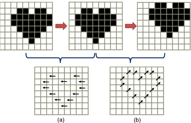
Optical flow is one of the basic motion estimation techniques exploited in many computer vision applications to examine the motion pattern of object. The idea of optical flow was introduced in 1950 by a psychologist named Gibson (Gibson, 1950). Optical flow was first proposed to describe the visual perception and stimulus experienced by an animal when it moves through the world. Later on, optical flow stimulus has been expanded for the perception by the human observers during their own movement through the environ-ment. It is the distribution of two-dimensional apparent motion of objects in an image based on the brightness patterns in an image (Horn & Schunck, 1981). It indicates the
Figure 2.9: Optical flow estimation of the moving object between temporally-consecutive images towards the directions of: (a) Left; (b)Upper right
displacement and velocity of each image pixel between temporally-consecutive images by assuming that the pixel intensity values are translated between subsequent pairs of frames (D. Fleet & Weiss, 2006). The displacement vector is known as optical flow vec-tor, expresses in terms of direction and magnitude. For example, Figure 2.9 illustrates the optical flow estimation of the moving object between adjacent frames.
Conventionally, there are several approaches to accomplish the optical flow compu-tation. They are broadly classified into the following four main types: (a) differential (i.e., Horn and Schunk (Horn & Schunck, 1981), Lucas and Kanade (Lucas & Kanade, 1981), Nagel (Nagel, 1983)); (b) region-based matching (i.e., Anandan (Anandan, 1987), Singh (Singh, 1990)); (c) energy-based (i.e., Heeger (Heeger, 1987)), and; (d) phase-based method (i.e., Fleet and Jepson (D. J. Fleet & Jepson, 1990)). To investigate and discover the capability of these four types of optical flow, Barron et al. (Barron et al., 1994) conducted the experiments by applying them in multiple video sequences. It is reported that the local differential method achieved the best performance over the other
three methods. As a result, differential method is opted to approximate the optical flow motion vectors in this thesis. The following descriptions and derivations of optical flow are discussed based on thedifferential method.
In general, five assumptions are made in order to estimate the optical flow: (a) bright-ness constancy - apparent brightbright-ness of the moving objects remains constant between frames as the changes in the pixel intensity are due solely to motion (highlights, shad-ows, variable illumination and surface translucency phenomena exists in the images are ignored); (b) object rigidity - the objects in the scene are rigid and the shape changes are neglected; (c) temporal persistence - motion of a surface patch changes gradually over time because the movement between two adjacent frames are small; (d) spatial coherence - the neighborhood of the object are likely to be situated on the same surface. Thus, the neighboring points of the object are having similar velocity values, and; (e) continuous and differentiable - image velocity are approximated from spatio-temporal derivatives of image intensities by using differential method. Therefore, image flow field is continuous and differentiable in both the space and time domains (Beauchemin & Barron, 1995).
The optical flow constraint equation is formulated as:
∇I•℘+It=0, (2.8)
whereI(x,y,t)represents the changes of temporal image brightness in intensity values with respect to time at point (x,y). ∇I = (Ix,Iy) is the spatial gradient and It is the temporal
gradient of the intensity functions. Assume that the point of interest in the image is initially positioned at (x,y). After a change in time by dt, it moves through a distance
(dx,dy). The horizontal and vertical components of the optical flow are denoted as:
℘= [p= dx
dt,q= dy dt]
Figure 2.10:Formation of HOOF with four bins
Optical flow has been employed in a variety of interesting applications, such as facial expression recognition (Kenji, 1991), human skeleton tracking (Schwarz et al., 2012), medical imaging (Garcia et al., 2012), vehicle detection (Dawood et al., 2013), object removal (Hamilton & Breckon, 2016) and many more. In addition, several variants of optical flow have been designed and optimized to best meet different research objectives. Histogram of Oriented Optical Flow (HOOF) (Chaudhry et al., 2009) is one of the techniques developed based on the optical flow. It was first introduced to recognize human actions by building activity profiles for each frame of a video. The optical flow values are captured as histogram bins because they are extremely vulnerable to the background changes and illumination variation. By doing so, it allows the feature representation to be independent to the direction of the motion and scale variation. To generate HOOF, optical flow for each pair of adjacent frames is first computed. Then, the orientation and magnitude are calculated based on the horizontal and vertical flow vectors. Lastly, the histogram is formed according to the orientation, with magnitude being used as the weight to highlight the importance of each optical flow. Figure 2.10 shows the formation of HOOF with bin number of four.

![Figure 2.4: Example of three different circularly symmetric neighbor sets, [P, R]: (a) [4,1]; (b) [8,1]; (c) [8,2]](https://thumb-us.123doks.com/thumbv2/123dok_us/971889.2627442/37.892.175.802.83.292/figure-example-different-circularly-symmetric-neighbor-sets-p.webp)